Regional Flux Inversion#
Bayesian Inversion for Regional CH₄ Emissions#
This notebook demonstrates solving a regional atmospheric inverse problem using Bayesian estimation.
Problem Setup#
State (x): Regional CH₄ flux anomalies on a spatial grid [µmol/m²/s]
Observations (z): CH₄ concentration enhancements at observation sites [ppm]
Forward model: z = H @ x (atmospheric transport from fluxes to concentrations)
Approach#
Synthetic Jacobian: Distance-based Gaussian sensitivity (flux → concentration)
Synthetic Truth: Gaussian emission hotspots within domain
Synthetic Observations: Concentrations from truth + noise
Bayesian Estimation: Recover fluxes from noisy concentration measurements
1. Imports#
[1]:
import matplotlib.pyplot as plt
import numpy as np
import pandas as pd

from fips.problems.flux import FluxProblem

# Configure plotting
plt.style.use("seaborn-v0_8-darkgrid")
%matplotlib inline
2. Configuration#
[2]:
# ==============================================================================
# RANDOM SEED
# ==============================================================================

RANDOM_SEED = 42

# ==============================================================================
# DOMAIN CONFIGURATION
# ==============================================================================

# Spatial domain (lat/lon bounds)
XMIN, XMAX = -112.0, -111.5  # longitude [deg]
YMIN, YMAX = 40.5, 41.0  # latitude [deg]
DX, DY = 0.05, 0.05  # grid spacing [deg]

# Time domain
T_START = pd.Timestamp("2024-01-01")
T_STOP = pd.Timestamp("2025-01-01")
STATE_FREQ = "MS"  # state frequency
OBS_FREQ = "D"  # observation frequency

# ==============================================================================
# OBSERVATION SITES
# ==============================================================================

N_SITES = 3  # number of observation locations

# ==============================================================================
# EMISSION HOTSPOTS (Truth field)
# ==============================================================================

N_HOTSPOTS = 2  # number of Gaussian emission centers
HOTSPOT_AMPLITUDE = 1.0  # peak flux [µmol/m²/s]
HOTSPOT_WIDTH = 0.1  # Gaussian width [deg] (std dev)

# ==============================================================================
# PRIOR CONFIGURATION
# ==============================================================================

PRIOR_MEAN = 0.05  # prior flux mean [µmol/m²/s]
PRIOR_STD_FRACTION = 0.5  # prior uncertainty as fraction of prior mean

# ==============================================================================
# JACOBIAN (SENSITIVITY)
# ==============================================================================

INFLUENCE_RADIUS = 0.3  # Gaussian influence radius [deg]

# ==============================================================================
# OBSERVATION ERROR
# ==============================================================================

OBS_NOISE_STD = 0.001  # observation noise [ppm]

print("Configuration:")
print(f"  Domain: [{XMIN}, {XMAX}] × [{YMIN}, {YMAX}] (spacing {DX}°)")
print(f"  Time: {T_START} to {T_STOP}")
print(f"  Observation sites: {N_SITES}")
print(f"  Hotspots: {N_HOTSPOTS} @ {HOTSPOT_AMPLITUDE} µmol/m²/s")
print(f"  Prior: {PRIOR_MEAN} ± {PRIOR_MEAN * PRIOR_STD_FRACTION} µmol/m²/s")
Configuration:
  Domain: [-112.0, -111.5] × [40.5, 41.0] (spacing 0.05°)
  Time: 2024-01-01 00:00:00 to 2025-01-01 00:00:00
  Observation sites: 3
  Hotspots: 2 @ 1.0 µmol/m²/s
  Prior: 0.05 ± 0.025 µmol/m²/s
3. Helper Functions#
[3]:
def build_grid(xmin, xmax, ymin, ymax, dx, dy):
    """
    Build spatial grid.

    Returns
    -------
    lons : array
        Longitude cell centers
    lats : array
        Latitude cell centers
    """
    lons = np.arange(xmin + dx / 2, xmax, dx)
    lats = np.arange(ymin + dy / 2, ymax, dy)
    return lons, lats


def build_obs_sites(n_sites, xmin, xmax, ymin, ymax, seed=42):
    """
    Generate random observation site locations within domain.

    Returns
    -------
    obs_lons : array
        Observation longitude coordinates
    obs_lats : array
        Observation latitude coordinates
    """
    np.random.seed(seed)
    obs_lons = np.random.uniform(xmin, xmax, n_sites)
    obs_lats = np.random.uniform(ymin, ymax, n_sites)
    return obs_lons, obs_lats


def gaussian_2d(x, y, x0, y0, sigma):
    """
    Evaluate 2D Gaussian.

    Parameters
    ----------
    x, y : array
        Coordinates (can be meshgrid)
    x0, y0 : float
        Gaussian center
    sigma : float
        Gaussian width

    Returns
    -------
    z : array
        Gaussian values
    """
    return np.exp(-0.5 * ((x - x0) ** 2 + (y - y0) ** 2) / sigma**2)


def build_truth_field(lons, lats, hotspots, amplitude, width):
    """
    Build synthetic truth field from Gaussian hotspots.

    Parameters
    ----------
    lons, lats : array
        Grid coordinates
    hotspots : list of (lon, lat)
        Hotspot center locations
    amplitude : float
        Peak flux amplitude
    width : float
        Gaussian width

    Returns
    -------
    flux : 2D array
        Flux field [n_lon × n_lat]
    """
    X, Y = np.meshgrid(lons, lats, indexing="ij")
    flux = np.zeros_like(X)

    for lon0, lat0 in hotspots:
        flux += amplitude * gaussian_2d(X, Y, lon0, lat0, width)

    return flux


def build_jacobian(obs_lons, obs_lats, state_lons, state_lats, influence_radius):
    """
    Build synthetic Jacobian using distance-based Gaussian sensitivity.

    H[i,j] = sensitivity of observation i to flux j
           = exp(-0.5 * (distance_ij / influence_radius)^2)

    Parameters
    ----------
    obs_lons, obs_lats : array
        Observation site coordinates
    state_lons, state_lats : array
        State grid coordinates
    influence_radius : float
        Gaussian influence radius

    Returns
    -------
    H : 2D array
        Jacobian [n_obs × n_state]
    """
    n_obs = len(obs_lons)
    n_lon = len(state_lons)
    n_lat = len(state_lats)
    n_state = n_lon * n_lat

    H = np.zeros((n_obs, n_state))

    idx = 0
    for i_lon in range(n_lon):
        for i_lat in range(n_lat):
            state_lon = state_lons[i_lon]
            state_lat = state_lats[i_lat]

            for i_obs in range(n_obs):
                # Great-circle distance (simplified for small distances)
                dlon = obs_lons[i_obs] - state_lon
                dlat = obs_lats[i_obs] - state_lat
                distance = np.sqrt(dlon**2 + dlat**2)

                # Gaussian sensitivity
                H[i_obs, idx] = np.exp(-0.5 * (distance / influence_radius) ** 2)

            idx += 1

    return H


print("Helper functions loaded.")
Helper functions loaded.
4. Build Domain and Observation Network#
[4]:
# Build grid
lons, lats = build_grid(XMIN, XMAX, YMIN, YMAX, DX, DY)
X_grid, Y_grid = np.meshgrid(lons, lats, indexing="ij")

n_lon = len(lons)
n_lat = len(lats)
n_state_spatial = n_lon * n_lat

print(f"Spatial grid: {n_lon} × {n_lat} = {n_state_spatial} cells")

# Generate observation sites
obs_lons, obs_lats = build_obs_sites(N_SITES, XMIN, XMAX, YMIN, YMAX, seed=RANDOM_SEED)
location_mapper = {}
print(f"Observation sites: {N_SITES}")
for i, (lon, lat) in enumerate(zip(obs_lons, obs_lats, strict=False)):
    print(f"  Site {i}: ({lon:.3f}, {lat:.3f})")
    location_mapper[i] = (lat, lon)

# Generate hotspot locations
np.random.seed(RANDOM_SEED + 1)
hotspot_lons = np.random.uniform(XMIN, XMAX, N_HOTSPOTS)
hotspot_lats = np.random.uniform(YMIN, YMAX, N_HOTSPOTS)
hotspots = list(zip(hotspot_lons, hotspot_lats, strict=False))

print(f"Hotspots: {N_HOTSPOTS}")
for i, (lon, lat) in enumerate(hotspots):
    print(f"  Hotspot {i}: ({lon:.3f}, {lat:.3f})")
Spatial grid: 10 × 10 = 100 cells
Observation sites: 3
  Site 0: (-111.813, 40.799)
  Site 1: (-111.525, 40.578)
  Site 2: (-111.634, 40.578)
Hotspots: 2
  Hotspot 0: (-111.942, 40.567)
  Hotspot 1: (-111.695, 40.620)
5. Build Time Grids#
[5]:
# State time bins (fluxes)
state_times = pd.date_range(
    start=T_START, end=T_STOP, freq=STATE_FREQ, inclusive="left"
)
n_time_state = len(state_times)

# Observation time bins
obs_times = pd.date_range(start=T_START, end=T_STOP, freq=OBS_FREQ, inclusive="left")
n_time_obs = len(obs_times)

print(f"State time bins: {n_time_state}")
for t in state_times:
    print(f"  {t}")

print(f"\nObservation times: {n_time_obs}")
print(f"  {obs_times[0]} to {obs_times[-1]}")
State time bins: 12
  2024-01-01 00:00:00
  2024-02-01 00:00:00
  2024-03-01 00:00:00
  2024-04-01 00:00:00
  2024-05-01 00:00:00
  2024-06-01 00:00:00
  2024-07-01 00:00:00
  2024-08-01 00:00:00
  2024-09-01 00:00:00
  2024-10-01 00:00:00
  2024-11-01 00:00:00
  2024-12-01 00:00:00

Observation times: 366
  2024-01-01 00:00:00 to 2024-12-31 00:00:00
6. Build Jacobian#
[6]:
print("Building Jacobian...")
H = build_jacobian(obs_lons, obs_lats, lons, lats, INFLUENCE_RADIUS)

print(f"Jacobian shape: {H.shape}")
print(f"  Range: [{H.min():.4f}, {H.max():.4f}]")
print(f"  Mean sensitivity: {H.mean():.4f}")
Building Jacobian...
Jacobian shape: (3, 100)
  Range: [0.1350, 0.9999]
  Mean sensitivity: 0.6698
7. Generate Synthetic Truth and Observations#
[7]:
# Build truth field with seasonal cycle
print("Building truth field with seasonal cycle...")
truth_2d = build_truth_field(lons, lats, hotspots, HOTSPOT_AMPLITUDE, HOTSPOT_WIDTH)

# Create time-varying truth with seasonal cycle
# Amplitude varies from 0.5x to 1.5x the base, peaking in summer (day ~180)
truth_3d = np.zeros((n_lon, n_lat, n_time_state))

for t_idx, t in enumerate(state_times):
    # Seasonal cycle: sinusoid with peak in summer
    # day_of_year: 0-365, peak amplitude at day ~180 (June-July)
    day_of_year = t.dayofyear
    seasonal_factor = 1.0 + 0.5 * np.sin(2 * np.pi * (day_of_year - 152) / 365.25)
    truth_3d[:, :, t_idx] = seasonal_factor * truth_2d

# Reshape to flat vector in the correct order: iterate over lon, lat, then time
truth_data = truth_3d.reshape(-1)

# Create state index to match this ordering
state_index = pd.MultiIndex.from_product(
    [lons, lats, state_times], names=["lon", "lat", "time"]
)

truth_series = pd.Series(truth_data, index=state_index, name="truth")

print(f"Truth field: mean={truth_series.mean():.4f}, max={truth_series.max():.4f}")
print(f"  Seasonal range: {truth_series.min():.4f} to {truth_series.max():.4f}")

# Prior (uniform, independent of season)
prior_series = pd.Series(PRIOR_MEAN, index=state_index, name="flux")
print(f"Prior field: {prior_series.mean():.4f} ± {PRIOR_MEAN * PRIOR_STD_FRACTION:.4f}")
Building truth field with seasonal cycle...
Truth field: mean=0.3525, max=1.5691
  Seasonal range: 0.0001 to 1.5691
Prior field: 0.0500 ± 0.0250
8. Generate Synthetic Observations#
[8]:
print("Generating synthetic observations...")

# For each observation time, compute concentrations from time-varying fluxes
syn_obs_data = []
syn_obs_index = []

for t_obs in obs_times:
    # Find nearest state time
    idx = np.searchsorted(state_times, t_obs, side="left")
    if idx >= n_time_state:
        idx = n_time_state - 1

    # Extract truth for this time step from the 3D array
    state_flat = truth_3d[:, :, idx].ravel()

    # Compute concentrations
    conc = H @ state_flat

    # Add noise
    noise = np.random.normal(0, OBS_NOISE_STD, N_SITES)
    conc_noisy = conc + noise

    syn_obs_data.extend(conc_noisy)
    for i_site in range(N_SITES):
        syn_obs_index.append((i_site, t_obs))

obs_index = pd.MultiIndex.from_tuples(syn_obs_index, names=["site_idx", "time"])
syn_obs = pd.Series(syn_obs_data, index=obs_index, name="concentration")

print(f"Observations: {len(syn_obs)}")
print(f"  Range: [{syn_obs.min():.6f}, {syn_obs.max():.6f}]")
print(f"  Mean: {syn_obs.mean():.6f}")
Generating synthetic observations...
Observations: 1098
  Range: [11.480887, 42.115867]
  Mean: 26.427648
9. Setup Inverse Problem#
[9]:
print("Setting up flux inversion problem...")

# Prior covariance (diagonal)
prior_std = PRIOR_MEAN * PRIOR_STD_FRACTION
S_0 = pd.DataFrame(
    np.diag((prior_std**2) * np.ones(len(prior_series))),
    index=state_index,
    columns=state_index,
)

# Observation covariance (diagonal)
S_z = pd.DataFrame(
    np.diag((OBS_NOISE_STD**2) * np.ones(len(syn_obs))),
    index=obs_index,
    columns=obs_index,
)

# Forward operator: map state (lon, lat, time_state) to obs (site, time_obs)
# The state_index is organized as: (lon[0], lat[0], t[0]), (lon[0], lat[0], t[1]), ...,
#                                   (lon[0], lat[1], t[0]), (lon[0], lat[1], t[1]), ...
# So for each observation at time t_obs, we need to find all spatial cells at the corresponding state time
H_full = np.zeros((len(syn_obs), len(prior_series)))

obs_row = 0
for t_obs in obs_times:
    # Find corresponding state time index
    state_time_idx = np.searchsorted(state_times, t_obs, side="left")
    if state_time_idx >= n_time_state:
        state_time_idx = n_time_state - 1

    # For each observation site at this time
    for site_idx in range(N_SITES):
        # Fill in Jacobian row for all spatial locations
        for lon_idx in range(n_lon):
            for lat_idx in range(n_lat):
                spatial_idx = lon_idx * n_lat + lat_idx
                col_pos = spatial_idx * n_time_state + state_time_idx
                H_full[obs_row, col_pos] = H[site_idx, spatial_idx]
        obs_row += 1

H_mat = pd.DataFrame(H_full, index=obs_index, columns=state_index)

# Create flux inversion problem
# The prepare functions will handle conversion of pandas objects to Vector/Matrix types
problem = FluxProblem(
    obs=syn_obs,
    prior=prior_series,
    forward_operator=H_mat,
    prior_error=S_0,
    modeldata_mismatch=S_z,
)

print("Flux inversion problem configured.")
print(f"  State dimension: {len(prior_series)}")
print(f"  Observation dimension: {len(syn_obs)}")
print(f"  Jacobian shape: {H_full.shape}")
Setting up flux inversion problem...
Flux inversion problem configured.
  State dimension: 1200
  Observation dimension: 1098
  Jacobian shape: (1098, 1200)
10. Solve#
[10]:
print("Solving...")
problem.solve(estimator="bayesian")
print("✓ Solution complete")
Solving...
✓ Solution complete
[11]:
problem.obs
[11]:
Vector(name='None', shape=(1098,))
block          site_idx  time
concentration  0         2024-01-01    19.783718
               1         2024-01-01    17.022029
               2         2024-01-01    20.813514
               0         2024-01-02    14.939326
               1         2024-01-02    12.854288
                                         ...
                         2024-12-30    22.693028
               2         2024-12-30    27.748752
               0         2024-12-31    26.374392
               1         2024-12-31    22.694512
               2         2024-12-31    27.747134
Name: None, Length: 1098, dtype: float64
11. Diagnostics#
[12]:
# Extract results
x_post = problem.posterior.data.values
z_obs_vals = problem.obs.data.values
z_post = problem.posterior_obs.data.values
z_prior = problem.prior_obs.data.values

# Posterior state diagnostics
print("POSTERIOR STATE (FLUX)")
print(f"  Mean: {x_post.mean():.4f} µmol/m²/s")
print(f"  Std:  {x_post.std():.4f} µmol/m²/s")
print(f"  Range: [{x_post.min():.4f}, {x_post.max():.4f}]")

# Observation fit
print("\nOBSERVATION FIT")
print(f"  RMSE: {problem.estimator.RMSE:.6e} ppm")
print(f"  R²: {problem.estimator.R2:.4f}")
residuals = z_obs_vals - z_post
print(f"  Max residual: {np.abs(residuals).max():.6e} ppm")

# Uncertainty reduction
prior_std_full = np.sqrt(np.diag(problem.prior_error.values))
post_std_full = np.sqrt(np.diag(problem.posterior_error.values))
reduction = (1 - post_std_full / prior_std_full) * 100

print("\nUNCERTAINTY REDUCTION")
print(f"  Mean: {reduction.mean():.1f}%")
print(f"  Range: [{reduction.min():.1f}%, {reduction.max():.1f}%]")

# Information content
print("\nINFORMATION CONTENT")
print(f"  DOFS: {problem.estimator.DOFS:.1f}")
print(f"  Reduced χ²: {problem.estimator.reduced_chi2:.3f}")
POSTERIOR STATE (FLUX)
  Mean: 0.3492 µmol/m²/s
  Std:  0.3724 µmol/m²/s
  Range: [-0.2208, 1.4783]

OBSERVATION FIT
  RMSE: 1.017315e-03 ppm
  R²: 1.0000
  Max residual: 5.317285e-03 ppm

UNCERTAINTY REDUCTION
  Mean: 1.5%
  Range: [0.7%, 3.2%]

INFORMATION CONTENT
  DOFS: 36.0
  Reduced χ²: 400.136
12. Visualization#
[13]:
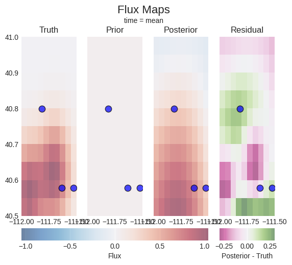
problem.plot.fluxes(truth=truth_series, sites=location_mapper)
[13]:
(<Figure size 640x480 with 6 Axes>,
 array([<Axes: title={'center': 'Truth'}>,
        <Axes: title={'center': 'Prior'}>,
        <Axes: title={'center': 'Posterior'}>,
        <Axes: title={'center': 'Residual'}>], dtype=object))
[14]:
problem.plot.concentrations(location_dim="site_idx")

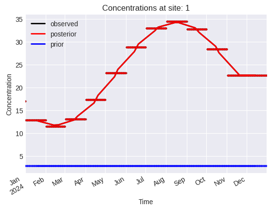
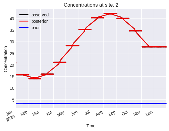
[14]:
array([<Axes: title={'center': 'Concentrations at site: 0'}, xlabel='Time', ylabel='Concentration'>,
       <Axes: title={'center': 'Concentrations at site: 1'}, xlabel='Time', ylabel='Concentration'>,
       <Axes: title={'center': 'Concentrations at site: 2'}, xlabel='Time', ylabel='Concentration'>],
      dtype=object)
[15]:
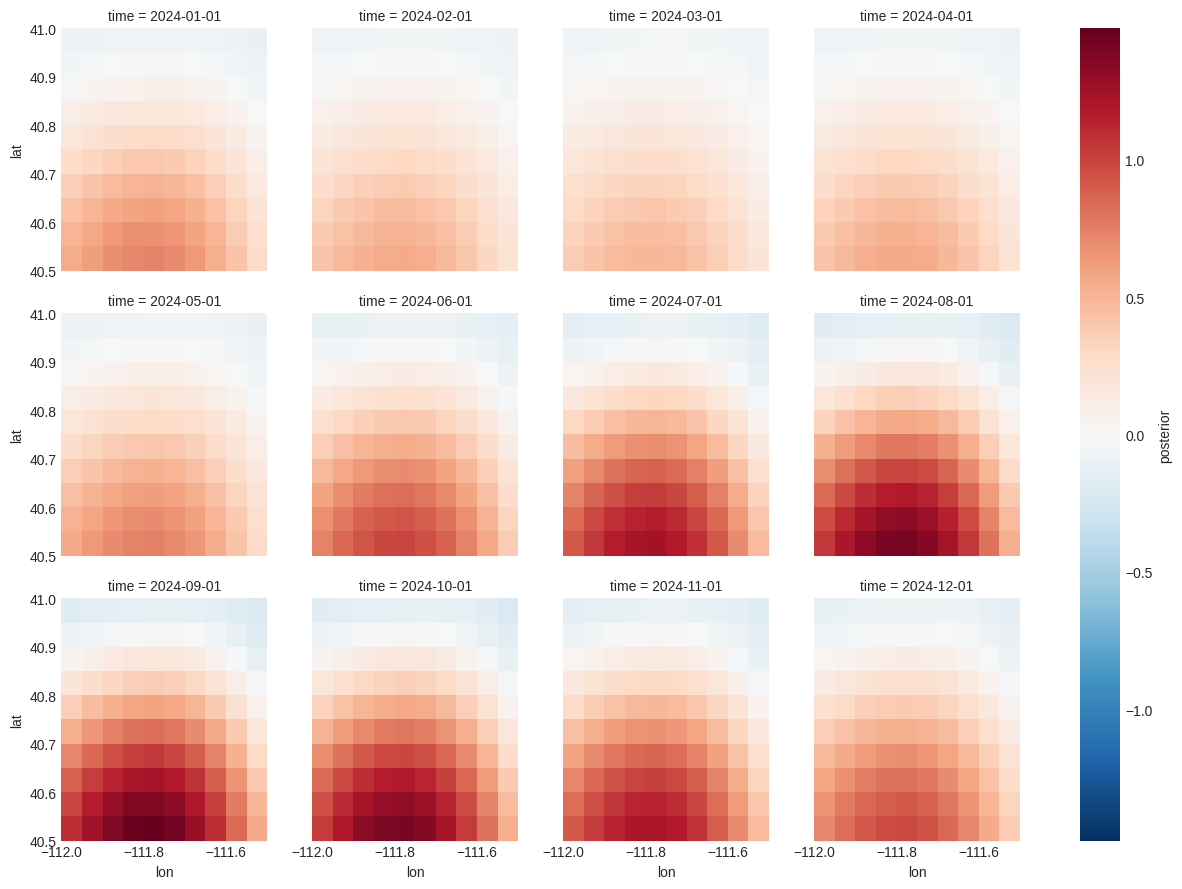
problem.posterior["flux"].to_xarray().plot(x="lon", y="lat", col="time", col_wrap=4)
[15]:
<xarray.plot.facetgrid.FacetGrid at 0x1471f84cd090>