Find sites and data#
Note
The examples under “Which sites measure what” use only the package’s configuration and run when the documentation is built. The output of the others is from runs on CHPC on 11 October 2026 (why it is recorded). The archive keeps growing, so the dates at the end of the data, and how long a call takes, will have moved on by the time you read this.
Before you read data, find out what there is: which sites measure the pollutant you want, and when they have data. The tables on Sites and instruments say which sites and instruments exist, what each measures and when each was installed. That is what the sites were set up to measure, not that there are data. This page shows the calls that answer both questions, and how recent the data are. When the answer is “nothing”, When there is nothing to read says what each error means.
I want to know |
Use |
|---|---|
Which sites measure CH4? |
|
What a site measures, and since when |
|
When a site has data, and at which level |
|
The newest data at a site |
|
One pollutant from several sites in one table |
|
Why a read failed or came back empty |
Which sites measure what#
The tables on Sites and instruments come from objects you can use yourself. The blocks in this section run when the documentation is built, so their output is current. A site object says what the site measures, and which instruments it has had:
In [1]: import uataq

In [2]: from uataq import Network

In [3]: site = uataq.get_site("WBB")

In [4]: site.config["name"], site.config["zagl"]
Out[4]: ('William Browning Building', 35)

In [5]: sorted(site.pollutants)
Out[5]: ['BC', 'CH4', 'CO', 'CO2', 'NO', 'NO2', 'NOX', 'O3', 'PM2.5']

In [6]: [instrument.name for instrument in site.instruments]
Out[6]:
['lgr_ugga',
 'magee_ae33',
 'metone_es642',
 'teledyne_t200',
 'teledyne_t300',
 'teledyne_t400',
 'teledyne_t500u',
 'teom_1400ab']

In [7]: site.instruments["teledyne_t400"].active_range
Out[7]: TimeRange(start=2016-08-29 00:00:00, stop=None)

In [8]: type(site.instruments["teledyne_t400"]).__name__
Out[8]: 'Teledyne_T400'
uataq.laboratory.sites lists every site ID, and site.config holds the
site’s own keys (see Configuration). repr(site), which is what a notebook
shows for site, prints the whole entry, with the notes of the instruments
that have one: why its dates are what they are, and where its data end.
Pollutant names are upper case (NOx is 'NOX' here), but you can type
them in any case when you read data. To go the other way and find the sites that
measure a pollutant, make a Network. A Network is a list of sites
and one pollutant, and it is how uataq asks a question across sites; "all"
is every site that measures the pollutant, and one site ID given as a string,
Network("WBB", "CO2"), is the network of that site, the same as
Network(["WBB"], "CO2"):
In [9]: Network("all", "CH4")
Out[9]: Network(sites=['CSP', 'FRU', 'HDP', 'HPL', 'LDF', 'ROO', 'TRX01', 'WBB'], pollutant='CH4')
CH4 is measured at fewer sites than CO2. Of these, WBB (on the University of
Utah campus) and LDF (the Salt Lake Valley landfill) are in the valley, HDP
(Hidden Peak) is in the Wasatch Mountains above it, CSP, FRU, HPL and ROO are in
the Uintah Basin, and TRX01 is a TRAX train. The site tables on
Sites and instruments give each site’s name and position.
The network’s sites attribute lists the same sites by ID, so a loop over
net.sites reaches only sites that measure the pollutant.
An instrument’s window, its active_range, says when it was installed, not
when it recorded data. That is why PM2.5 is in WBB’s list although both of
WBB’s PM2.5 instruments, metone_es642 and teom_1400ab, have an end date:
In [10]: print("\n".join(f"{i.name:15} {i.active_range}" for i in site.instruments))
lgr_ugga        After 2013-10-09 00:00:00
magee_ae33      2020-07-29 00:00:00 to 2024-06-20 00:00:00
metone_es642    2017-03-07 00:00:00 to 2022-06-08 00:00:00
teledyne_t200   After 2017-01-19 00:00:00
teledyne_t300   After 2017-05-03 00:00:00
teledyne_t400   After 2016-08-29 00:00:00
teledyne_t500u  2020-07-29 00:00:00 to 2023-01-25 00:00:00
teom_1400ab     2016-09-22 00:00:00 to 2017-03-02 00:00:00
When a site has data#
The examples below read the archive on CHPC, and start from these lines:
>>> import uataq
>>> from uataq import Network
>>> wbb = uataq.get_site("WBB")
Network.get_availability() tells you when sites have data for a pollutant.
Give it a time range and it returns a table with one row for each stretch of
time that has data:
>>> net = Network(["WBB", "CSP", "HDP"], "CH4")
>>> avail = net.get_availability(["2024-01-01", None], freq="W", lvls=["final"])
>>> avail
   SID    lvl      start       stop
0  WBB  final 2024-01-01 2024-11-25
1  WBB  final 2024-12-02 2026-10-19
2  CSP  final 2024-01-01 2024-12-16
3  CSP  final 2024-12-30 2026-10-12
4  HDP  final 2024-01-01 2025-02-10
Each row is one site (SID), one data level (lvl) and one stretch from
start up to, but not including, stop. The times are UTC, like the data.
Between two rows of the same site there is a gap with no data: WBB has none for
the week starting 2024-11-25, and CSP has none for the two weeks starting
2024-12-16. HDP’s last row stops on 2025-02-10, and nothing follows it: HDP has
no data after that. A site with no data in the range has no rows at all. A
stop can fall after the day of the run (this one was on 12 October 2026): the
last weekly bin, from 12 to 19 October, holds the data up to the run.
To get the first and last date for each site:
>>> avail.groupby("SID").agg(first=("start", "min"), last=("stop", "max"))
         first       last
SID
CSP 2024-01-01 2026-10-12
HDP 2024-01-01 2025-02-10
WBB 2024-01-01 2026-10-19
last is the end of the final bin (see below), not the time of the last
measurement. With weekly bins it can be up to a week later.
Mobile sites (TRX01 and the others) work the same way. For an instrument
that two research groups log, the call checks both archives, so it can show data
that a read from one group would not return.
Bins#
The call cuts time into bins, one week here (freq="W"), and a bin counts as
having data if any measurement of the pollutant falls in it. So a coarse bin
hides a short gap. WBB logged no CO2 at all on 4 March 2024. Daily bins
(the default) show it, and weekly bins do not:
>>> co2 = Network(["WBB"], "CO2")
>>> co2.get_availability("2024-03", lvls=["final"])
   SID    lvl      start       stop
0  WBB  final 2024-03-01 2024-03-04
1  WBB  final 2024-03-05 2024-03-24
2  WBB  final 2024-03-25 2024-04-01
>>> co2.get_availability("2024-03", freq="W", lvls=["final"])
   SID    lvl      start       stop
0  WBB  final 2024-02-26 2024-04-01
The weekly row starts on 2024-02-26 because weeks start on Monday. A bin at
either end of the range can reach past it. freq is a pandas period alias:
"D" (day), "W" (week) or "M" (month).
Levels#
By default the call checks all four data levels (raw, qaqc,
calibrated and final; see The four levels) and gives each bin the
highest level that has data in it. A stretch labeled
qaqc was therefore measured, but the final level has nothing for it. WBB
has no final CO2 for August 2021:
>>> co2.get_availability("2021", freq="M", lvls=["qaqc", "final"])
   SID    lvl      start       stop
0  WBB  final 2021-01-01 2021-08-01
1  WBB   qaqc 2021-08-01 2021-09-01
2  WBB  final 2021-09-01 2022-01-01
get_obs() always reads the final level, so it has nothing to return for
that month (see When there is nothing to read).
A level has data in a bin when a row has a value in a _cal or a _raw
column (see Column names), the columns Network.get_obs() returns.
TRX01’s lgr_ugga_manual_cal fills only _raw, and its months
count as final.
How long it takes#
get_availability opens and reads every data file in the range. That is the
only way to know a pollutant was measured: a file can exist and hold nothing for
the pollutant you asked about. It is quick for a few sites and a short range, and
slow for everything. These times are for WBB CO2, from one process on a CHPC
compute node on 26 October 2026:
Call |
Time |
|---|---|
Two years (2024 and 2025), all four levels, daily bins (the defaults) |
146 s |
The same, with |
8.3 s |
The same, with |
8.3 s |
The year 2025 alone, one level: |
4 s, 10 s, 13 s, 31 s |
The defaults again, with |
36 s |
So:
Ask for the levels you need with
lvls. Therawlevel has far more files than the others and takes about seven times as long asfinal.Give a time range. With no
time_rangethe call covers every year the site has data.The bin size hardly matters for the time. Pick it for the question.
Use more processes for many sites.
num_processesspreads the files over that many processes, and"max"uses every core you were given. Checking CO2 at all 19 sites that measure it, every year, final level only, took 73 s withnum_processes=8(11 October 2026). Do this in a Slurm job, not on a login node.
The script below makes the figure in the next section. It has the __main__
guard (see A year or more). Save it as availability.py:
import uataq


def main():
    net = uataq.Network("all", "CO2")
    avail = net.get_availability(freq="M", lvls=["qaqc", "final"], num_processes=8)
    ax = net.plot_availability(avail)
    ax.figure.savefig("co2_availability.png", dpi=100, bbox_inches="tight")


if __name__ == "__main__":
    main()
Then submit it in a job. Take the job script under Use uataq in a Slurm job and
change three things: add #SBATCH --cpus-per-task=8 (a core for each process),
set --mem=16G, and end with python availability.py. That job took 7
minutes, and the figure below is what it drew.
A picture#
Network.plot_availability() draws the table: a row for each site, time
along the bottom, and a bar wherever there is data, shaded by level. It needs
matplotlib. Pass it the table you already have, so a change of style does not
read the archive again.
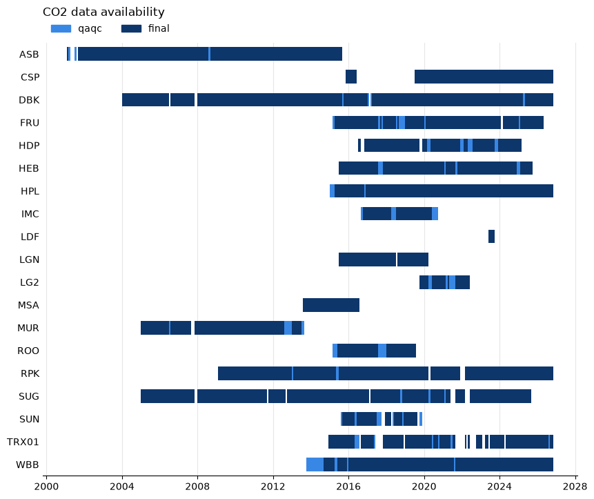
CO2 at every site that measures it, from the run above. Dark bars are final data and light bars are qaqc data with nothing in final.#
The newest data#
get_recent_obs() returns the last few days of a site. It reads the same
level as get_obs(), and returns the same kind of table. The default is
10 days:
>>> obs = uataq.get_recent_obs("WBB", pollutants="CO2")
>>> print(obs.shape)
(82846, 3)
>>> obs.tail(3)
                     CO2d_ppm_cal  CO2d_ppm_raw instrument
Time_UTC
2026-10-29 22:33:10    453.085968      456.4526   lgr_ugga
2026-10-29 22:33:20    453.350899      456.7222   lgr_ugga
2026-10-29 22:33:30    453.269853      456.6404   lgr_ugga
Name the pollutants. With the default pollutants="all", ten days at WBB came
back as 1.3 million rows.
recent is a datetime.timedelta or any text pandas reads as a time span,
such as "3D", "3 days" or "12h":
>>> obs = uataq.get_recent_obs("WBB", recent="3D", pollutants="CO2")
>>> print(obs.index.min(), obs.index.max())
2026-10-26 23:51:53 2026-10-29 22:33:30
The last row is the newest data the archive holds at that level. This run was at 23:51 UTC on 29 October, and the newest WBB CO2 row was from 22:33 UTC the same day, so the data were about an hour and a quarter behind. A site that has stopped reporting has nothing recent and raises an error (HDP, under When there is nothing to read).