Which observations constrain a regional total?

An inversion’s answer is often one number: the emissions of a region over a year. This notebook asks how uncertain that number is before and after the observations, what each site contributes to it, and which of a few candidate sites would tighten it most. Every number is exact for the linear Gaussian problem and comes from the posterior already solved: nothing is solved again.

The setup is the one of the regional flux inversion, shortened: a year of monthly fluxes on a 10 x 10 grid, daily concentrations at three sites, a prior correlated in time and space. The observation error is five times larger here (0.01 ppm), so that no single site decides the answer.

import matplotlib.pyplot as plt
import numpy as np
import pandas as pd
import scipy.sparse as sp

import fips

rng = np.random.default_rng(42)

The problem

footprints builds the forward operator’s rows for any sites and days: each day a site sees the cells around a point upwind of it, in that day’s month. The same function will make the rows of the candidate sites.

lons = np.round(np.arange(-111.975, -111.5, 0.05), 3)
lats = np.round(np.arange(40.525, 41.0, 0.05), 3)
months = pd.date_range("2024-01-01", periods=12, freq="MS")
days = pd.date_range("2024-01-01", "2024-12-31", freq="D")
cells = pd.MultiIndex.from_product([months, lats, lons], names=["time", "lat", "lon"])
prior = fips.Vector.from_series(pd.Series(0.05, index=cells), block="flux")
grid_lat, grid_lon = np.meshgrid(lats, lons, indexing="ij")


def footprints(sites, days, rng):
    """Return the forward operator of daily concentrations at `sites` (a frame of lon, lat)."""
    labels = pd.MultiIndex.from_product([sites.index, days], names=["site", "obs_time"])
    rows, cols, values = [], [], []
    upwind = rng.normal(0.0, 0.1, (len(labels), 2))
    for i, (site, day) in enumerate(labels):
        x = sites.at[site, "lon"] + upwind[i, 0]
        y = sites.at[site, "lat"] + upwind[i, 1]
        distance = np.hypot(grid_lon - x, grid_lat - y)
        rows.append(np.full(grid_lat.size, i))
        cols.append((day.month - 1) * grid_lat.size + np.arange(grid_lat.size))
        values.append(np.exp(-0.5 * (distance.ravel() / 0.15) ** 2))
    matrix = sp.csr_array(
        (np.concatenate(values), (np.concatenate(rows), np.concatenate(cols))),
        shape=(len(labels), len(cells)),
    )
    space = fips.Space({"concentration": labels})
    return fips.Operator(matrix, space, prior.space)


sites = pd.DataFrame(  # the three sites of the regional example, placed by hand
    {"lon": [-111.85, -111.7, -111.55], "lat": [40.6, 40.85, 40.7]},
    index=pd.Index(["site_a", "site_b", "site_c"], name="site"),
)
forward = footprints(sites, days, rng)
noise = 0.01  # ppm
obs = fips.Vector(
    forward.data @ np.full(len(cells), 0.05)
    + 1.9
    + rng.normal(0.0, noise, forward.shape[0]),
    forward.rows,
)
problem = fips.Problem(
    prior=prior,
    prior_cov=fips.Kronecker(
        fips.Exponential("time", "60D"),
        fips.Exponential(["lat", "lon"], 20.0, metric="haversine"),
    ).with_std(0.25),
    obs=obs,
    obs_cov=fips.Independent().with_std(noise),
    forward=forward,
    offset=1.9,
)
post = fips.solve(problem)
post.summary()[["n_state", "n_obs", "dofs"]]

	n_state	n_obs	dofs
0	1200	1098	225.470576

The totals: the region’s year, its months, and a seasonal difference

The region is the eastern half of the grid. fips.aggregate.sum builds the aggregation W from the state’s own levels: by a yearly pd.Grouper on the time and a Series that maps the eastern longitudes to "east", and dropna=True leaves out the western cells, which the Series does not map. The months of the region are the same with a monthly grouping.

east = pd.Series(
    "east", index=pd.Index(lons[lons > -111.75], name="lon"), name="region"
)
annual = fips.aggregate.sum(
    prior.space, by=[pd.Grouper(level="time", freq="YS"), east], dropna=True
)
monthly = fips.aggregate.sum(prior.space, by=["time", east], dropna=True)
annual.rows, monthly.rows

(Space(flux: 1 x ['time', 'region']), Space(flux: 12 x ['time', 'region']))

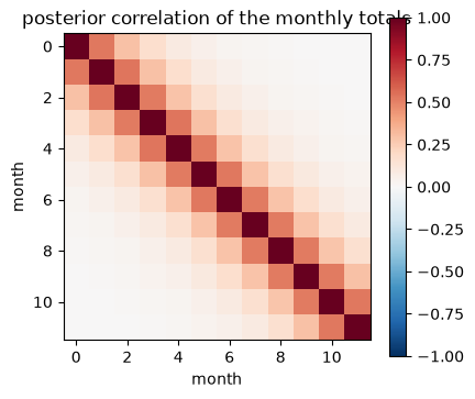
A combination of totals is one more row: the summer (June to August) minus the winter (December to February), C @ monthly, with C the weights of the months. Its uncertainty uses the covariance between the months, which the posterior has; their standard deviations alone could not give it.

month = monthly.rows.select("flux").get_level_values("time").month
weights = np.where(np.isin(month, [6, 7, 8]), 1.0, 0.0) - np.where(
    np.isin(month, [12, 1, 2]), 1.0, 0.0
)
summer_minus_winter = (
    fips.Operator(
        weights[None, :],
        fips.Space({"seasonal": pd.Index(["JJA - DJF"], name="what")}),
        monthly.rows,
    )
    @ monthly
)
table = pd.concat([post.uncertainty(annual), post.uncertainty(summer_minus_winter)])
table.index = ["annual total", "summer - winter"]
table.round(3)

	prior_std	posterior_std	reduction
annual total	51.281	1.037	0.980
summer - winter	24.108	0.523	0.978

post.uncertainty gives each row’s standard deviation before the observations (prior_std, from problem.prior_cov.aggregate(W)) and after (posterior_std, from post.cov(W)), and the fraction the observations take off. The months’ posterior errors are correlated, which is what the seasonal difference’s standard deviation takes into account:

months_cov = post.cov(monthly).dense()
sd = np.sqrt(np.diag(months_cov))
correlation = months_cov / np.outer(sd, sd)
fig, ax = plt.subplots(figsize=(4.5, 4))
im = ax.imshow(correlation, vmin=-1, vmax=1, cmap="RdBu_r")
ax.set_xlabel("month")
ax.set_ylabel("month")
ax.set_title("posterior correlation of the monthly totals")
fig.colorbar(im, ax=ax);

What each site contributes

post.data_worth(by="site", W=annual) takes each site out in turn (a rank update of the posterior covariance, exact, with no new solve) and gives the total’s standard deviation without the site and with it, the fraction the site takes off on top of the other two (reduction), and the site’s share of the degrees of freedom for signal. std_alone and reduction_alone are the standard deviation and the fraction with only this site’s observations added to the prior, where reduction is on top of all the other sites.

by_site = post.data_worth(by="site", W=annual)
by_site.droplevel(["block", "time", "region"]).round(3)

	n_obs	dofs	std_without	std_with	reduction	std_alone	reduction_alone
site
site_a	366	78.582	1.169	1.037	0.113	2.440	0.952
site_b	366	80.864	1.116	1.037	0.071	1.423	0.972
site_c	366	66.025	1.208	1.037	0.142	1.509	0.971

The shares of DOFS of the three sites sum to the problem’s DOFS:

by_site.groupby(level="site")["dofs"].first().sum(), post.dofs

(np.float64(225.4705755130525), 225.4705755071374)

Any level of the observations groups them, a time bin too: which months of observations matter most for the annual total?

by_month = post.data_worth(by=pd.Grouper(level="obs_time", freq="MS"), W=annual)
reduction = by_month["reduction"].droplevel(["block", "time", "region"])
reduction.index = reduction.index.strftime("%b")
ax = reduction.plot.bar(figsize=(7, 3))
ax.set_ylabel("reduction of the annual total's std")
ax.set_xlabel("month of observations removed");

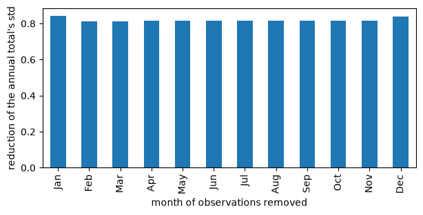
Without one month of observations, the annual total loses most of what the observations gave it: here a day’s concentration sees only the fluxes of its own month, so that month’s fluxes fall back toward the prior, held only by the prior’s 60-day correlation with the months around it.

Which candidate site would help most

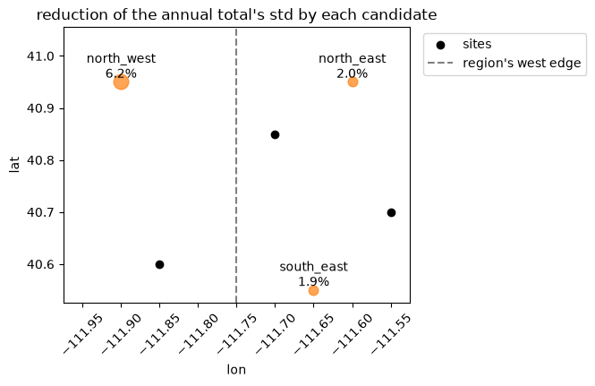
Candidate observations are their rows of the forward operator and the covariance of their errors, no values. Three candidate sites, observed daily with the same error as the others: post.candidate_worth adds each on its own, by the same kind of update, and gives the same columns. The best candidate for the eastern total need not be one of the eastern sites: the table, not the map, says which.

candidates = pd.DataFrame(
    {"lon": [-111.6, -111.9, -111.65], "lat": [40.95, 40.95, 40.55]},
    index=pd.Index(["north_east", "north_west", "south_east"], name="site"),
)
H_new = footprints(candidates, days, rng)
worth = post.candidate_worth(
    H_new, fips.Independent().with_std(noise), by="site", W=annual
)
worth.droplevel(["block", "time", "region"]).round(3)

	n_obs	dofs	std_without	std_with	reduction
site
north_east	366	49.114	1.037	1.016	0.020
north_west	366	60.430	1.037	0.973	0.062
south_east	366	43.673	1.037	1.017	0.019

fig, ax = plt.subplots(figsize=(5, 4))
ax.scatter(sites["lon"], sites["lat"], color="black", label="sites")
for name, row in candidates.iterrows():
    gain = worth.xs(name, level="site")["reduction"].iloc[0]
    ax.scatter(
        row["lon"], row["lat"], s=2000 * gain + 20, color="tab:orange", alpha=0.7
    )
    ax.annotate(
        f"{name}\n{gain:.1%}", (row["lon"], row["lat"]), ha="center", va="bottom"
    )
ax.axvline(-111.75, color="gray", linestyle="--", label="region's west edge")
ax.set_xlim(lons.min(), lons.max())
ax.set_ylim(lats.min(), lats.max() + 0.08)
ax.set_xlabel("lon")
ax.set_ylabel("lat")
ax.set_title("reduction of the annual total's std by each candidate")
ax.tick_params(axis="x", labelrotation=45)
ax.legend(loc="upper left", bbox_to_anchor=(1.02, 1));

The numbers are exact for this problem: solving it again with a candidate’s observations added gives the same standard deviation. Here, the check for one:

name = "north_east"
keep = H_new.rows.select("concentration").get_level_values("site") == name
labels = problem.obs.space.select("concentration").append(
    H_new.rows.select("concentration")[keep]
)
space = fips.Space({"concentration": labels})
bigger = fips.Problem(
    prior=prior,
    prior_cov=problem.prior_cov,
    obs=fips.Vector(np.concatenate([obs.values, np.zeros(keep.sum())]), space),
    obs_cov=fips.Independent().with_std(noise),
    forward=fips.Operator(
        sp.vstack([forward.sparse(), H_new.sparse()[keep]]).tocsr(), space, prior.space
    ),
    offset=1.9,
)
again = np.sqrt(fips.solve(bigger).cov(annual).variances.values)
np.c_[worth.xs(name, level="site")["std_with"].to_numpy(), again]

array([[1.01625949, 1.01625949]])

Notes

• A site that repeats what another sees shows little on top of it (reduction) but a lot alone (reduction_alone): site_b adds 7 % to the other two, yet by itself takes 97 % off the prior’s std. The two answer different questions: what is lost if the site is dropped, and what the site is worth by itself. To see what two sites that repeat each other give together, remove both (a coarser by).

• candidate_worth adds each group to the problem as it is; for a network of several new sites, give them one group label.

• The candidates’ errors are taken to be independent of the problem’s observations, and are divided by gamma as the problem’s are.