
User Guide#
This guide takes fips’s objects one at a time, in the order a problem uses them, and says what each is for before how to call it. A First Problem solves one problem from start to finish; Terminology defines the words.
Spaces and vectors#
Every number in fips has a label, and fips matches numbers by their labels,
never by their position. A Space is the labels of a state, of
the observations, or of one axis of a matrix: an ordered set of named
blocks, each labeled by its own pandas index. A state can have a flux
block labeled by (time, lat, lon) and a bias block labeled by
site; the observations a station block and a satellite block.
A Vector is values on a space: a prior, the observations, an
estimate. It comes from a Series (one block) or from several (one per block):
In [1]: import numpy as np

In [2]: import pandas as pd

In [3]: import fips

In [4]: cells = pd.Index([1, 2, 3], name="cell")

In [5]: sites = pd.Index(["north", "south"], name="site")

In [6]: prior = fips.Vector.from_blocks(
   ...:     {"flux": pd.Series([1.0, 2.0, 0.5], index=cells), "bias": pd.Series(0.0, index=sites)},
   ...:     name="prior",
   ...: )
   ...:

In [7]: prior.to_series()
Out[7]:
block  cell  site
flux   1     nan      1.0
       2     nan      2.0
       3     nan      0.5
bias   NaN   north    0.0
             south    0.0
Name: prior, dtype: float64

In [8]: prior["flux"].to_series()
Out[8]:
block  cell
flux   1       1.0
       2       2.0
       3       0.5
Name: prior, dtype: float64
Together, the blocks are one pandas.MultiIndex with the block
level first (prior.space.index). A level that one block has and another
lacks is missing (NaN) on the other’s rows, and Space is the one
place that adds and removes those levels: prior["flux"] comes back labeled
as it was given, integer cells and all. prior.space.select("flux") gives a
block’s labels, and to_xarray() a DataArray on the levels of
one block (a Dataset for several).
Labels are kept as they are given: fips does not convert strings to numbers or
round floats. Duplicate, missing (NaN) and unnamed labels raise a
ValueError that names them. Labels that should match only after
rounding are rounded on purpose, with round_labels() (also
on a Space and an Operator).
A vector is read-only: a new value is a new vector. align()
puts a vector in the order of a space with the same labels, and
combine_first() fills the labels one vector lacks from
another (the estimate of part of the state, completed by the prior).
Operators#
An Operator is a matrix with a space on each axis: the forward
operator (observations by state), an aggregation, a gain. Its matrix is kept
in the cheapest form that is exact (a dense array, a SciPy sparse matrix, a
diagonal, Kronecker factors; see Linear Algebra), and the labels are
beside it. There are three ways in:
Operator(matrix, rows, cols)labels a matrix you have, by position: its rows arerows’s labels in order, its columnscols’s. A SciPy sparse matrix stays sparse.Operator.from_framereads a labeled DataFrame, dense or with pandas-sparse columns.Operator.from_blocksassembles one from its blocks, each named by its row block and its column block: a DataFrame, or a tuple(matrix, row_labels, col_labels). Given the spaces (rows=,cols=), it places each block by its labels: a label the block has no entry for is zero, as a pair of blocks left out is, and a label the space does not have raises.
In [9]: obs_id = pd.Index(["o1", "o2", "o3"], name="obs_id")

In [10]: obs = fips.Vector.from_series(pd.Series([2.0, 3.5, 1.0], index=obs_id), block="co2")

In [11]: H = fips.Operator.from_blocks(
   ....:     {
   ....:         ("co2", "flux"): pd.DataFrame(np.eye(3), index=obs_id, columns=cells),
   ....:         ("co2", "bias"): pd.DataFrame([[1.0, 0.0], [1.0, 0.0], [0.0, 1.0]], index=obs_id, columns=sites),
   ....:     },
   ....:     rows=obs.space,
   ....:     cols=prior.space,
   ....: )
   ....:

In [12]: H.to_frame()
Out[12]:
block        flux            bias
cell            1    2    3   NaN
site          nan  nan  nan north south
block obs_id
co2   o1      1.0  0.0  0.0   1.0   0.0
      o2      0.0  1.0  0.0   1.0   0.0
      o3      0.0  0.0  1.0   0.0   1.0

In [13]: (H @ prior).to_series()
Out[13]:
block  obs_id
co2    o1        1.0
       o2        2.0
       o3        0.5
dtype: float64
H @ vector is a vector, H @ other an operator, and + and - add
operators; each first matches the labels they meet on, in any order, and a
label on one side only raises. H["co2", "flux"] is one block, H.T the
transpose, and to_frame() the dense DataFrame.
Sparse matrices. A forward operator from atmospheric transport is mostly
zeros. An operator built
from a scipy.sparse matrix (or from a DataFrame with pandas-sparse
columns) keeps it sparse, and so do the products and sums that stay mostly
zeros: a diagonal or sparse matrix times a sparse one is sparse, and a product
is dense once more than a quarter of its entries are filled, or when either
side is dense. The forward operator, the prior covariance and the observation
covariance can each be dense or sparse:
In [14]: import scipy.sparse as sp

In [15]: J = sp.random(3, 3, density=0.4, random_state=0, format="csr")

In [16]: sparse_H = fips.Operator(J, obs.space, fips.Space({"flux": cells}))

In [17]: sparse_H.data
Out[17]: <3x3 SparseOperator with dtype=float64>
A large product of a sparse matrix and a dense one (\(H S_0 H^T\) with a
dense \(S_0\) has one) runs on threads, each multiplying a block of the
sparse matrix’s rows, and gives the same numbers as one thread, bit for bit. It
uses the CPUs the process may run on (a Slurm job’s --cpus-per-task, not the
node’s), and no more than OMP_NUM_THREADS when that is set, as NumPy’s BLAS
does: OMP_NUM_THREADS=1 keeps it on one thread.
Covariances and covariance models#
A Covariance is a symmetric operator from a space to itself:
the prior covariance \(S_0\) or the observation covariance \(S_z\). It
adds what a covariance needs: its variances,
solve(), logdet(),
quadratic_form() (of its inverse) and
sqrt(), each done the way its form makes cheap.
A matrix you give (fips.Covariance(array, space),
from_frame(), from_blocks(), or the
variances of Covariance.diagonal) is checked
once, when the covariance is built: it must be symmetric, to 1e-10 of its
largest entry, and positive semidefinite, with no eigenvalue below zero by
more than roundoff (n * eps times the largest). One that is not, a
covariance estimated or tapered by hand, say, raises, naming its smallest
eigenvalue. The check is the square root a draw is made with
(sample()), built and kept: for a dense matrix, one
Cholesky factorization and an n x n factor held beside it; for a sparse
one, a factor for each group of correlated rows; for a singular matrix (zero
variances, a Constant block), which has no Cholesky factor, an
eigendecomposition. A covariance a model builds is positive semidefinite by
construction and is not checked.
Independent errors are a diagonal, kept as its variances, one number per
element: Covariance.diagonal takes a scalar
(one variance for every element), an array (one each) or a vector. Independent
parts go side by side with Covariance.block_diag, each keeping its form:
In [18]: S_0 = fips.Covariance.block_diag(
   ....:     fips.Covariance.diagonal(0.25, fips.Space({"flux": cells})),
   ....:     fips.Covariance.diagonal(0.01, fips.Space({"bias": sites})),
   ....: )
   ....:

In [19]: S_0.variances.to_series()
Out[19]:
block  cell  site
flux   1     nan      0.25
       2     nan      0.25
       3     nan      0.25
bias   NaN   north    0.01
             south    0.01
Name: variance, dtype: float64

In [20]: S_0.data
Out[20]: <5x5 DiagonalOperator with dtype=float64>
Covariance models. Correlated errors are usually written as a correlation model and the standard deviations. A correlation model says how correlated two labels are from their values on some levels:
Exponential,GaussianandMaterndecay with the distance along their levels: a datetime level with a time scale (Exponential("time", "30D")), numeric levels as a straight line, or latitude and longitude on the Earth (metric="haversine", the great-circle distance in km;metric="chordal", through the Earth, which a Gaussian or a Matérn needs to stay positive-definite). The two levels are read by position, not by name, so give latitude first:Exponential(["lat", "lon"], 10.0, metric="haversine");Constantis 1 everywhere, andIndependentthe identity (1 for a label with itself, 0 otherwise);Kroneckermultiplies models on separate levels, kept as its factors.
model.with_std(std) is the covariance. With the standard deviations as a
number, or a pandas Series on the block’s labels (lined up by label), it is a
covariance model, which build(space) puts on a space; a plain array is
refused, since it has no labels. A Problem builds its
covariance models on the prior’s or the observations’ space itself. With a
Vector of standard deviations, the space is known and it is a
Covariance at once. Covariance models add (a + b), and
block_diag() takes them by block name.
within= keeps a model inside groups of labels and makes it zero between
them, as a sparse matrix: within=["site", "obs_time.date"] correlates the
observations of one site on one day only ("obs_time.date" is the date of
the obs_time level), and within="time.hour" the same hour of day only.
Here an independent instrument error plus an error correlated over 2 hours
within a site’s day:
In [21]: hours = pd.date_range("2024-01-01 21:00", periods=4, freq="h")

In [22]: labels = pd.MultiIndex.from_product([["A", "B"], hours], names=["site", "obs_time"])

In [23]: obs_cov = fips.Independent().with_std(0.1) + fips.Exponential(
   ....:     "obs_time", "2h", within=["site", "obs_time.date"]
   ....: ).with_std(0.5)
   ....:

In [24]: obs_cov
Out[24]: Independent().with_std(0.1) + Exponential(levels=('obs_time',), within=('site', 'obs_time.date'), scale=Timedelta('0 days 02:00:00'), metric='euclidean').with_std(0.5)

In [25]: obs_cov.build(fips.Space({"co2": labels})).dense().round(3)
Out[25]:
array([[0.26 , 0.152, 0.092, 0.   , 0.   , 0.   , 0.   , 0.   ],
       [0.152, 0.26 , 0.152, 0.   , 0.   , 0.   , 0.   , 0.   ],
       [0.092, 0.152, 0.26 , 0.   , 0.   , 0.   , 0.   , 0.   ],
       [0.   , 0.   , 0.   , 0.26 , 0.   , 0.   , 0.   , 0.   ],
       [0.   , 0.   , 0.   , 0.   , 0.26 , 0.152, 0.092, 0.   ],
       [0.   , 0.   , 0.   , 0.   , 0.152, 0.26 , 0.152, 0.   ],
       [0.   , 0.   , 0.   , 0.   , 0.092, 0.152, 0.26 , 0.   ],
       [0.   , 0.   , 0.   , 0.   , 0.   , 0.   , 0.   , 0.26 ]])
A Kronecker model is kept as its factors: its covariance holds a
KroneckerOperator, which never forms the
\(n \times n\) matrix. Each factor is evaluated once, on the unique values
of its levels, and the labels can be any subset of the product, in any order:
In [26]: state = pd.MultiIndex.from_product(
   ....:     [pd.date_range("2024-01-01", periods=4, freq="7D"), [40.5, 40.6], [-112.0, -111.9]],
   ....:     names=["time", "lat", "lon"],
   ....: )
   ....:

In [27]: prior_cov = fips.Kronecker(
   ....:     fips.Exponential("time", "14D"),
   ....:     fips.Exponential(["lat", "lon"], 10.0, metric="haversine"),
   ....: ).with_std(0.5)
   ....:

In [28]: S = prior_cov.build(fips.Space({"flux": state}))

In [29]: [factor.shape for factor in S.data.factors]
Out[29]: [(4, 4), (4, 4)]
A new kind of correlation is a subclass of
CorrelationModel: a frozen dataclass with its
levels and a correlation(coords) method.
The problem#
A Problem is the question: the prior and its covariance, the
observations and theirs, the forward operator, and an optional offset. It
checks the labels once, when it is built, by an exact join: the forward
operator’s rows and the observation covariance must have exactly the labels of
the observations, its columns and the prior covariance exactly those of the
prior, in any order. A block or a label on one side only raises a
ValueError naming it, so nothing is filled with zeros and nothing is
rounded without your asking. Each input is then held in the order of the
prior’s and the observations’ spaces, in its own form.
The offset \(c\) is the part of the observations the state does not
explain (a background): a vector on the observations’ space, or one number.
predict() is \(H x + c\) for any state, such as the
prior or a truth:
In [30]: problem = fips.Problem(
   ....:     prior=prior,
   ....:     prior_cov=S_0,
   ....:     obs=obs,
   ....:     obs_cov=fips.Independent().with_std(0.2),
   ....:     forward=H,
   ....:     offset=0.5,
   ....: )
   ....:

In [31]: problem.predict(problem.prior).to_series()
Out[31]:
block  obs_id
co2    o1        1.5
       o2        2.5
       o3        1.0
dtype: float64
A problem is not changed by a solve, and makes other problems from itself.
Aggregated observations. Problem.aggregate
gives the problem of aggregated observations: the observations, the forward
operator, the observation covariance and the offset each go through one
aggregation \(W\) (\(W z\), \(W H\), \(W S_z W^T\),
\(W c\)). fips.aggregate.mean() and fips.aggregate.sum() build
\(W\) from the labels, grouped by levels, time bins or a mapping. Here,
hourly observations at two sites become daily means:
In [32]: rng = np.random.default_rng(0)

In [33]: hours = pd.date_range("2024-01-01", periods=48, freq="h")

In [34]: labels = pd.MultiIndex.from_product([["A", "B"], hours], names=["site", "obs_time"])

In [35]: ch4 = fips.Vector.from_series(pd.Series(rng.normal(2.0, 0.1, 96), index=labels), block="ch4")

In [36]: flux = fips.Vector.from_series(pd.Series(1.0, index=pd.Index(["c0", "c1", "c2"], name="cell")), block="flux")

In [37]: hourly = fips.Problem(
   ....:     prior=flux,
   ....:     prior_cov=fips.Independent().with_std(0.5),
   ....:     obs=ch4,
   ....:     obs_cov=fips.Independent().with_std(0.05),
   ....:     forward=fips.Operator(rng.uniform(0, 0.1, (96, 3)), ch4.space, flux.space),
   ....: )
   ....:

In [38]: daily = hourly.aggregate(
   ....:     fips.aggregate.mean(ch4.space, by=["site", pd.Grouper(level="obs_time", freq="1D")])
   ....: )
   ....:

In [39]: daily.obs.to_series()
Out[39]:
block  site  obs_time
ch4    A     2024-01-01    1.988586
             2024-01-02    2.025302
       B     2024-01-01    2.012840
             2024-01-02    2.020259
dtype: float64
Offsets the data should decide. An offset that is not known (a background
that drifts, a calibration bias) is a block of the state instead:
fips.offset_block() gives one offset per group of observations, zeros as
their prior, and the forward block that adds each offset to its observations.
Their prior covariance is any model on their labels; here the days of a site
are correlated:
In [40]: days = pd.interval_range(hours[0], periods=2, freq="1D", closed="left", name="obs_time")

In [41]: offsets, H_offsets = fips.offset_block(ch4.space, by=[days, "site"])

In [42]: with_offsets = fips.Problem(
   ....:     prior=fips.Vector.from_blocks({"flux": flux, "offset": offsets}),
   ....:     prior_cov=fips.Covariance.block_diag(
   ....:         flux=fips.Independent().with_std(0.5),
   ....:         offset=fips.Exponential("obs_time", "2D", within="site").with_std(0.1),
   ....:     ),
   ....:     obs=ch4,
   ....:     obs_cov=fips.Independent().with_std(0.05),
   ....:     forward=fips.Operator.from_blocks(
   ....:         {("ch4", "flux"): hourly.forward, ("ch4", "offset"): H_offsets["ch4", "offset"]}
   ....:     ),
   ....: )
   ....:

In [43]: fips.solve(with_offsets).estimate["offset"].to_series().round(3)
Out[43]:
block   obs_time    site
offset  2024-01-01  A       1.831
                    B       1.838
        2024-01-02  A       1.864
                    B       1.876
Name: estimate, dtype: float64
Part of the state held at its prior. Problem.restrict solves for part of the state (cells no observation
sees well are left out) and holds the rest at its prior: their contribution
\(H x_0\) moves into the offset. combine_first() puts
the estimate back on the whole state:
In [44]: small = hourly.restrict(fips.Space({"flux": pd.Index(["c0", "c1"], name="cell")}))

In [45]: fips.solve(small).estimate.combine_first(hourly.prior).to_series().round(3)
Out[45]:
block  cell
flux   c0      14.828
       c1      17.424
       c2       1.000
Name: estimate, dtype: float64
Solving and the posterior#
fips.solve() solves a problem with a method and returns a
Posterior, the answer. The method is "analytic" by default
(the closed-form Gaussian posterior, the one method so far;
fips.available_methods() lists them), and its one option is the
regularization factor gamma. An unknown method or option raises with the
names it knows.
The analytic method factors the problem once, in one of two forms that give
the same posterior. The whitened form works in the observations’ size: it
whitens with the Cholesky factor of \(S_z\) (or the square root of its
diagonal), so \(S_z\) must be positive-definite, and factors the
\(m \times m\) matrix \(H S_0 H^T\) in that metric. It computes
\(H S_0\) in the forms of \(H\) and \(S_0\) (through the factors of
a Kronecker covariance), and the estimate, the variances, the DOFS and the
chi-squared from the factors, without forming anything \(n \times n\). The
information form works in the state’s size: it factors an
\(n \times n\) matrix built from \(H\), a square root of \(S_0\) and
\(S_z^{-1}\), and forms no \(m \times m\) matrix of its own (a dense
\(S_z\) is applied through its Cholesky factor, a Kronecker one through
its factors). It is used when there are fewer state elements than
observations and \(S_z\) is dense, diagonal, sparse, block diagonal or
Kronecker; otherwise the whitened form. In both, the full posterior
covariance (post.cov()), the gain and the averaging kernel are formed
only when they are read, once each. fips.solve() factors that matrix
by Cholesky at its gamma, the cheapest way to solve at one gamma; the
first post.with_gamma eigendecomposes it, which holds at any gamma,
and keeps it, so a sweep over gamma pays for one eigendecomposition.
In [46]: rng = np.random.default_rng(1)

In [47]: obs_labels = pd.MultiIndex.from_product([["conc"], range(15)], names=["block", "obs_id"])

In [48]: forward = fips.Operator.from_frame(
   ....:     pd.DataFrame(rng.uniform(0, 1, (15, len(state))), index=obs_labels, columns=state),
   ....:     col_block="flux",
   ....: )
   ....:

In [49]: problem = fips.Problem(
   ....:     prior=fips.Vector.from_series(pd.Series(1.0, index=state), block="flux"),
   ....:     prior_cov=prior_cov,
   ....:     obs=fips.Vector.from_series(pd.Series(rng.normal(3.0, 1.0, 15), index=obs_labels)),
   ....:     obs_cov=fips.Independent().with_std(0.7),
   ....:     forward=forward,
   ....: )
   ....:

In [50]: post = fips.solve(problem)

In [51]: post.variances.to_series().head()
Out[51]:
block  time        lat   lon
flux   2024-01-01  40.5  -112.0    0.134190
                         -111.9    0.143158
                   40.6  -112.0    0.117721
                         -111.9    0.124034
       2024-01-08  40.5  -112.0    0.096764
Name: variance, dtype: float64
How much the observations tell. dofs is the trace
of the averaging kernel, the number of independent pieces of information the
observations give about the state; dofs_per_element is
its diagonal on the state’s labels, so the share of a week, a region or a block
is a sum over its labels. information_content is the
Shannon information content, \(-\tfrac{1}{2} \ln \lvert I - A \rvert\) in
nats: where DOFS counts a constrained direction as at most 1, it keeps growing
as the observations get more precise. Both are read from the factors, without
the \(n \times n\) kernel:
In [52]: post.dofs_per_element.to_series().groupby(level="time").sum().round(3)
Out[52]:
time
2024-01-01    1.078
2024-01-08    1.033
2024-01-15    1.105
2024-01-22    1.134
Name: dofs_per_element, dtype: float64

In [53]: round(post.dofs, 3), round(post.information_content, 3)
Out[53]: (4.35, 4.772)
The posterior of aggregates. An aggregation \(W\) of the state (one row
per total or mean) gives the posterior covariance of the aggregates,
post.cov(W) (\(W \hat{S} W^T\)), their prior covariance,
problem.prior_cov.aggregate(W) (\(W S_0 W^T\)), and their averaging
kernel, post.averaging_kernel(W) (\(W A W^*\), with \(W^*\) the
pseudo-inverse of \(W\)), none forming the \(n \times n\) matrices.
uncertainty() puts the two standard deviations of each
aggregate side by side, with the fraction the observations take off. Here, the
total flux of each week:
In [54]: W = fips.aggregate.sum(problem.prior.space, by="time")

In [55]: post.cov(W).to_frame().round(4)
Out[55]:
block                  flux
time             2024-01-01 2024-01-08 2024-01-15 2024-01-22
block time
flux  2024-01-01     0.6225    -0.0449    -0.2583    -0.2736
      2024-01-08    -0.0449     0.3485    -0.1119    -0.1523
      2024-01-15    -0.2583    -0.1119     0.4141    -0.0257
      2024-01-22    -0.2736    -0.1523    -0.0257     0.5088

In [56]: post.uncertainty(W).round(3)
Out[56]:
                  prior_std  posterior_std  reduction
block time
flux  2024-01-01      1.416          0.789      0.443
      2024-01-08      1.416          0.590      0.583
      2024-01-15      1.416          0.643      0.546
      2024-01-22      1.416          0.713      0.496

In [57]: post.averaging_kernel(W).dense().diagonal().round(3)
Out[57]: array([0.488, 0.549, 0.488, 0.586])
A row of \(W\) is any linear combination of the state, so a combination of
totals is a row too: C @ W, with C the weights of the rows of W. Its
uncertainty includes the covariance between the totals: the change from one
week to the next is not the root of the two weeks’ variances summed:
In [58]: change = fips.Operator(
   ....:     np.array([[-1.0, 1.0, 0.0, 0.0]]),
   ....:     fips.Space({"change": pd.Index(["week 2 - week 1"], name="what")}),
   ....:     W.rows,
   ....: )
   ....:

In [59]: post.uncertainty(change @ W).round(3)
Out[59]:
                        prior_std  posterior_std  reduction
block  what
change week 2 - week 1      1.256           1.03       0.18
dropna=True on fips.aggregate.sum() and mean()
picks part of the state: labels a key cannot place are left out instead of
raising (a Series that maps only a region’s cells gives the region’s total, an
interval of one year that year’s), and so are the blocks not named in
blocks (a bias block next to the fluxes).
Another gamma or other observations, without a new solve. The factors
depend neither on gamma nor on the values of the observations, so
post.with_gamma(g) is fips.solve(problem, gamma=g) at the cost of a few
products, and post.with_data(obs) the posterior of other observations at
the same labels (a bootstrap, synthetic observations of a known truth). A sweep over gamma factors once, and the rows of
summary() stack:
In [60]: pd.concat([post.with_gamma(g).summary() for g in (0.25, 1.0, 4.0)], ignore_index=True)
Out[60]:
   gamma  n_state  n_obs      dofs  information_content       chi2  reduced_chi2        r2      rmse  \
0   0.25       16     15  2.256343             2.553364  12.424450      0.828297  0.082316  0.888671
1   1.00       16     15  4.350110             4.772422  26.420686      1.761379  0.522039  0.703456
2   4.00       16     15  7.290068             8.784718  58.434926      3.895662  0.727697  0.522095

   uncertainty_reduction
0               0.217130
1               0.314634
2               0.446752
What each group of observations adds. data_worth()
groups the observations by any of their levels (a site, a platform’s block, a
month by pd.Grouper), as desroziers() does, and says
for each group how uncertain each aggregate would be without it
(std_without) and is with it (std_with), the fraction it takes off on
top of the other observations (reduction), and its share of DOFS. Removing
a group is a rank update of \(\hat{S}\), exact for any model-data
mismatch, so no problem is solved again. Two columns say what the group is
worth by itself: std_alone is how uncertain the aggregate would be with only
this group’s observations, on the prior, and reduction_alone the fraction
that takes off the prior (a rank update of \(S_0\)). The two readings
differ when groups see the same part of the state: a site that adds little on
top of the others may have taught a lot had it been the only one. They agree
only when there is one group. The alone columns use the group’s own block of the
model-data mismatch, so they leave out its correlation with the other groups’
errors. For the total flux of the hourly problem above, observed at two sites:
In [61]: hourly_post = fips.solve(hourly)

In [62]: total = fips.aggregate.sum(hourly.prior.space, by=pd.Series("all", index=hourly.prior.space.select("flux"), name="region"))

In [63]: hourly_post.data_worth(by="site", W=total).round(3)
Out[63]:
                   n_obs   dofs  std_without  std_with  reduction  std_alone  reduction_alone
site block region
A    flux  all        48  1.445        0.132     0.093      0.292      0.131            0.849
B    flux  all        48  1.340        0.131     0.093      0.287      0.132            0.848
Observations that are not in the problem, a candidate site or platform, are
their rows of the forward operator and the covariance of their errors (no
values): candidate_worth() adds each group on its own,
by the same kind of update, and gives the same columns but the two alone ones
(a candidate is always added on top of the problem’s observations), so a network
design question (“which candidate site helps the total most”) is one call:
In [64]: new_sites = fips.Space({"ch4": pd.MultiIndex.from_product([["C", "D"], hours], names=["site", "obs_time"])})

In [65]: H_new = fips.Operator(rng.uniform(0, 0.1, (96, 3)), new_sites, flux.space)

In [66]: hourly_post.candidate_worth(H_new, fips.Independent().with_std(0.05), by="site", W=total).round(3)
Out[66]:
                   n_obs   dofs  std_without  std_with  reduction
site block region
C    flux  all        48  0.846        0.093     0.079      0.158
D    flux  all        48  0.879        0.093     0.077      0.174
Checking the covariances. desroziers() compares the
observation error variances the residuals diagnose with those the solve used,
per observation or averaged over groups; reduced_chi2
is near 1 when the covariances are right; leverage()
says which observations weigh most on a state.
chi2_tests() makes the reduced chi-squared a test
(Rodgers, 2000, chapter 12), and adds the same test of three more vectors:
each is compared with its own covariance, and has its degrees of freedom and
p-value, small when the vector is larger than the covariances allow and near 1
when it is smaller. The four rows are the innovation \(z - H x_0 - c\)
(the row of chi2, with \(m\) degrees of freedom),
the residual \(z - H \hat{x} - c\) (also \(m\)), the modeled increment
\(H (\hat{x} - x_0)\) and the increment \(\hat{x} - x_0\) (each with
as many degrees of freedom as the directions of the state the observations
constrain). In a linear problem, the only kind fips solves, the rows come in
two pairs of the same numbers: the residual’s test gives the innovation’s, the
modeled increment’s the increment’s. They differ only when the estimate is not
linear in the observations; the table has four rows so that it keeps its shape
when such a method comes. In the weekly problem the state has more elements
than its 15 observations, which constrain 15 directions of it, so all four rows
are the same number; in the hourly problem many observations see three state
elements, and the two increments have three degrees of freedom. Every test of
the hourly problem rejects its covariances (p-values of 0): its made-up
observations are much farther from the prior than its covariances allow.
In [67]: post.chi2_tests().round(3)
Out[67]:
                     chi2  dof  reduced_chi2  p_value
test
innovation         26.421   15         1.761    0.034
residual           26.421   15         1.761    0.034
modeled_increment  26.421   15         1.761    0.034
increment          26.421   15         1.761    0.034

In [68]: hourly_post.chi2_tests().round(3)
Out[68]:
                        chi2  dof  reduced_chi2  p_value
test
innovation         13671.719   96       142.414      0.0
residual           13671.719   96       142.414      0.0
modeled_increment   1393.446    3       464.482      0.0
increment           1393.446    3       464.482      0.0
Synthetic truth and observations#
To test an inversion on data whose answer you know, make the data from the
problem. Problem.simulate returns (truth,
obs), two vectors: a truth drawn from the prior, \(x \sim N(x_0, S_0)\),
and the observations it would give, \(z = H x + c + e\) with \(e \sim
N(0, S_z)\); predict() is the same without the error. Its
draws are Covariance.sample, which draws from
\(N(0, S)\) without forming \(S\) where its form has a cheaper root.
rng is a seed or a numpy.random.Generator (one generator passed to
every call gives independent trials), and a truth= of your own (another
inventory, 1.5 times the prior, on the prior’s labels in any order) replaces
the draw. A trial is the solve on other data, post.with_data(obs), one
product, so a Monte Carlo is a loop you write. If the inversion is honest, the
95% interval of each total holds the truth in about 95% of the trials:
In [69]: rng = np.random.default_rng(0)

In [70]: sd = np.sqrt(post.cov(W).variances.values)  # what the posterior claims

In [71]: inside = []

In [72]: for _ in range(500):
   ....:     truth, obs = problem.simulate(rng)
   ....:     estimate = post.with_data(obs).estimate
   ....:     inside.append(np.abs((W @ estimate).values - (W @ truth).values) <= 1.96 * sd)
   ....:

In [73]: np.mean(inside, axis=0).round(2)
Out[73]: array([0.97, 0.94, 0.94, 0.96])
The estimate is linear in the observations, so the loop has an exact answer:
post.recovery gives, for each total, the
mean and spread of the error and the probability that the interval holds the
truth, without sampling. post.recovery(world, W=W) does the same for data
from another world on the same labels, and truth= fixes the truth, as in
simulate. A variance below zero by roundoff is a standard deviation of 0;
one further below zero comes only from a covariance that is not positive
semidefinite, and is NaN, with a warning:
In [74]: post.recovery(W=W)[["truth", "estimate", "std", "posterior_std", "coverage"]].round(3)
Out[74]:
                  truth  estimate    std  posterior_std  coverage
block time
flux  2024-01-01    4.0       4.0  0.789          0.789      0.95
      2024-01-08    4.0       4.0  0.590          0.590      0.95
      2024-01-15    4.0       4.0  0.643          0.643      0.95
      2024-01-22    4.0       4.0  0.713          0.713      0.95
The data come from a world, and the inversion you run on them has its own assumptions. There are four kinds of world:
The problem itself:
problem.simulate(rng), as above, tests that the inversion is honest.A chosen truth:
problem.simulate(rng, truth=inventory)tests how much of another inventory the inversion recovers.Another observing system: a separate
Problemwith other observations and its own solve, compared on the uncertainty of the totals.One input wrong: the
Problemyour own code builds with one input changed (a background, the mismatch), thenworld.simulate(rng)andpost.with_data(obs), which solves its data with your assumptions.
Plotting#
fips draws one plot, plot_comparison() (the viz
extra): several vectors or Series on one axes, with a band of one standard
deviation from each covariance, and an optional truth. Maps and anything else
are drawn from to_series() and
to_xarray() with pandas, xarray or matplotlib:
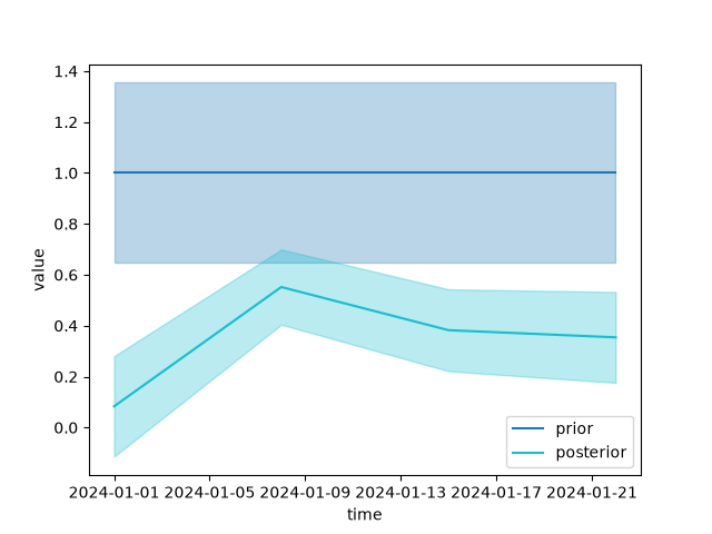
In [75]: from fips.visualization import plot_comparison

In [76]: weekly = fips.aggregate.mean(problem.prior.space, by="time")

In [77]: fig, ax = plot_comparison(
   ....:     (weekly @ problem.prior).to_series().droplevel("block").rename("prior"),
   ....:     (weekly @ post.estimate).to_series().droplevel("block").rename("posterior"),
   ....:     errors=[problem.prior_cov.aggregate(weekly), post.cov(weekly)],
   ....: )
   ....:
Example: a flux inversion#
fips knows no science domain: an atmospheric flux inversion is a
Problem whose state has a flux block and whose observations
a concentration block (any names will do), solved with fips.solve()
like any problem, with its blocks read by name:
import fips

problem = fips.Problem(
    prior=fips.Vector.from_series(prior_fluxes, block="flux"),
    prior_cov=prior_cov,  # a Covariance or a covariance model
    obs=fips.Vector.from_series(concentrations, block="concentration"),
    obs_cov=obs_cov,  # a Covariance or a covariance model
    forward=jacobian,  # an Operator: the transport Jacobian
    offset=background,  # a Vector on the observations, or a number
)
post = fips.solve(problem)

post.estimate["flux"].to_xarray()  # posterior fluxes on (time, lat, lon)
post.cov()["flux", "flux"]  # their posterior covariance
post.modeled_obs["concentration"]  # H x̂ + c
problem.predict(problem.prior)  # H x₀ + c
post.summary()  # DOFS, chi-squared, R², RMSE, ... as one row
For a STILT Jacobian, PYSTILT sums the
footprints onto your flux grid and time bins, as a sparse matrix with its row
and column labels. It has columns only for the cells a footprint touched,
while a problem needs the forward operator on exactly the prior’s labels:
Operator.from_blocks places it on the whole
state by its labels, and keeps it sparse:
import stilt

project = stilt.Project("my_project")
J = project.jacobian(project.simulations, grid, time_bins)
jacobian = fips.Operator.from_blocks(
    {("concentration", "flux"): (J.data, J.receptors.rename("receptor"), J.columns)},
    rows=obs.space,
    cols=prior.space,
)
Label the observations and the prior to match the Jacobian’s rows (receptor
ids) and columns ((time, lon, lat)).
Repeated inversions, logging and saving#
A workflow run many times (an inversion per month, a sweep over settings) is a
few functions in your own code: one that builds the Problem from
your settings, then fips.solve():
import pandas as pd

import fips

def build_problem(config) -> fips.Problem:
    """Load the observations and the prior, build H and the covariances."""
    ...

rows = [fips.solve(build_problem(config)).summary() for config in configs]
table = pd.concat(rows, ignore_index=True)
fips prints nothing. It logs through the standard logging module, under
the fips logger (the solve under fips.methods), and Python shows only
warnings until logging is configured; to see its INFO records:
import logging

logging.basicConfig(level=logging.INFO)
A Problem and a Posterior pickle with the
standard library (pickle.dump(post, file)): a posterior keeps its problem,
its options and what the method kept from the solve, and rebuilds every output
when it is read.