A regional flux inversion

Methane measured at a few sites depends on the emissions upwind of them. This notebook finds a year of monthly methane fluxes on a 10 x 10 grid from daily concentrations at three sites. The data are synthetic: a known truth (two emission hotspots with a seasonal cycle) makes the observations, so the estimate can be compared with it.

In the words of the terminology:

• the state is the flux of each grid cell in each month (µmol/m²/s), a block named flux labeled by (time, lat, lon);

• the observations are daily concentrations at each site (ppm), a block named concentration labeled by (site, obs_time);

• the forward operator is the transport: how much a unit flux in a cell raises the concentration at a site (here a made-up footprint that decays with distance), and it is sparse, since a day sees only its own month;

• the offset is the background concentration the fluxes do not explain;

• the prior is a uniform flux, with a prior covariance correlated in time and in space, and the observation covariance is independent noise.

import matplotlib.pyplot as plt
import numpy as np
import pandas as pd
import scipy.sparse as sp

import fips
from fips.visualization import plot_comparison

rng = np.random.default_rng(42)

The grid, the sites and the times

lons = np.round(np.arange(-111.975, -111.5, 0.05), 3)
lats = np.round(np.arange(40.525, 41.0, 0.05), 3)
months = pd.date_range("2024-01-01", periods=12, freq="MS")
days = pd.date_range("2024-01-01", "2024-12-31", freq="D")

sites = pd.DataFrame(
    {"lon": rng.uniform(-112.0, -111.5, 3), "lat": rng.uniform(40.5, 41.0, 3)},
    index=pd.Index(["site_a", "site_b", "site_c"], name="site"),
)
sites

	lon	lat
site
site_a	-111.613022	40.848684
site_b	-111.780561	40.547089
site_c	-111.570701	40.987811

Labels and vectors

The state is a flux for every month and cell, labeled by (time, lat, lon); the prior is a uniform 0.05 µmol/m²/s, in a block named flux. The observations are labeled by (site, obs_time), in a block named concentration.

cells = pd.MultiIndex.from_product([months, lats, lons], names=["time", "lat", "lon"])
prior = fips.Vector.from_series(
    pd.Series(0.05, index=cells, name="prior"), block="flux"
)

obs_labels = pd.MultiIndex.from_product([sites.index, days], names=["site", "obs_time"])
len(cells), len(obs_labels)

(1200, 1098)

The forward operator

A day’s concentration at a site sees only the fluxes of that day’s month, so most of the matrix is zero, and it is built sparse. Each day, a site sees the cells around a point upwind of it (the wind changes from day to day), and its sensitivity to a cell decays with the distance from that point. fips.Operator labels the matrix by position: rows in the order of obs_labels, columns in the order of cells.

grid_lat, grid_lon = np.meshgrid(
    lats, lons, indexing="ij"
)  # in the order of `cells` within a month
n_cells = grid_lat.size
rows, cols, values = [], [], []
upwind = rng.normal(
    0.0, 0.1, (len(obs_labels), 2)
)  # degrees, one shift per site and day
for i, (site, day) in enumerate(obs_labels):
    x, y = sites.at[site, "lon"] + upwind[i, 0], sites.at[site, "lat"] + upwind[i, 1]
    distance = np.hypot(grid_lon - x, grid_lat - y)
    month = day.month - 1
    rows.append(np.full(n_cells, i))
    cols.append(month * n_cells + np.arange(n_cells))
    values.append(np.exp(-0.5 * (distance.ravel() / 0.15) ** 2))
jacobian = sp.csr_array(
    (np.concatenate(values), (np.concatenate(rows), np.concatenate(cols))),
    shape=(len(obs_labels), len(cells)),
)

obs_space = fips.Space({"concentration": obs_labels})
forward = fips.Operator(jacobian, obs_space, prior.space)
forward.data

<1098x1200 SparseOperator with dtype=float64>

A truth, and the observations it makes

Two hotspots with a seasonal cycle, peaking in summer. The observations are the forward operator times the truth, plus a background of 1.9 ppm, plus noise.

hotspots = [(-111.8, 40.75), (-111.6, 40.6)]
spatial = sum(
    np.exp(-0.5 * ((grid_lon - x) ** 2 + (grid_lat - y) ** 2) / 0.1**2)
    for x, y in hotspots
)
season = 1.0 + 0.5 * np.sin(2 * np.pi * (months.day_of_year - 80) / 365.25)
truth = fips.Vector(
    np.concatenate([s * spatial.ravel() for s in season]), prior.space, name="truth"
)

background = 1.9
noise = 0.002
observed = forward @ truth
obs = fips.Vector(
    observed.values + background + rng.normal(0.0, noise, len(obs_labels)),
    obs_space,
    name="observed",
)

The covariances

The prior’s errors are alike for nearby cells and nearby months: a Kronecker product of an exponential correlation in time (over 60 days) and one in space (over 20 km along the great circle), with a standard deviation of 0.25 µmol/m²/s. It is kept as its two factors, never as the 1200 x 1200 matrix. The observation errors are independent.

prior_cov = fips.Kronecker(
    fips.Exponential("time", "60D"),
    fips.Exponential(["lat", "lon"], 20.0, metric="haversine"),
).with_std(0.25)
obs_cov = fips.Independent().with_std(noise)

The problem and its solution

The background is the problem’s offset: the part of the observations the fluxes do not explain.

problem = fips.Problem(
    prior=prior,
    prior_cov=prior_cov,
    obs=obs,
    obs_cov=obs_cov,
    forward=forward,
    offset=background,
)
post = fips.solve(problem)
post.summary()

	gamma	n_state	n_obs	dofs	information_content	chi2	reduced_chi2	r2	rmse	uncertainty_reduction
0	1.0	1200	1098	280.013506	1179.232066	995.421281	0.906577	1.0	0.001724	0.632659

Maps

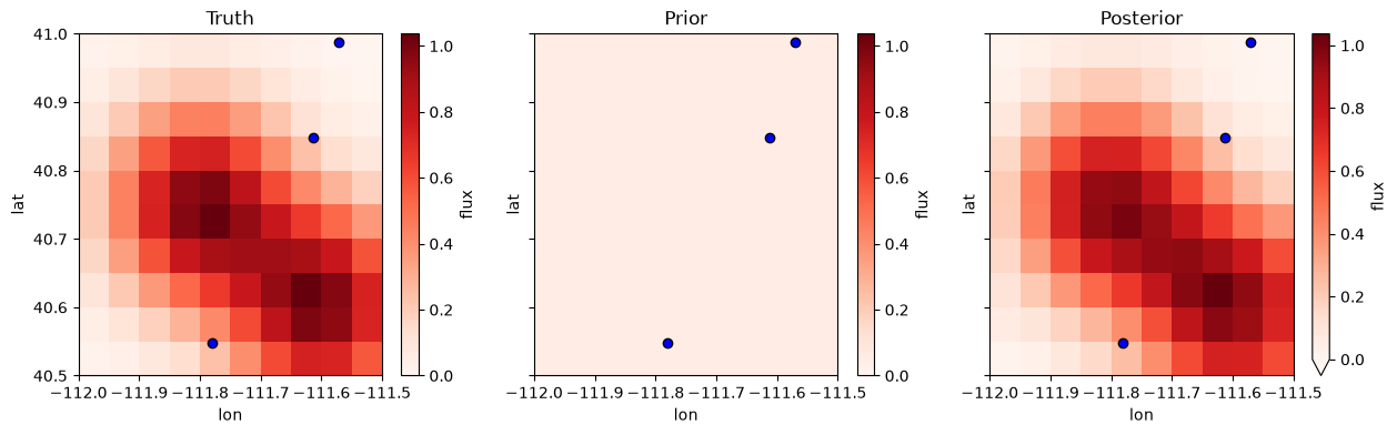
to_xarray() puts the flux block on its levels, (time, lat, lon), so the yearly means are one line each.

means = {
    "Truth": truth["flux"].to_xarray().mean("time"),
    "Prior": problem.prior["flux"].to_xarray().mean("time"),
    "Posterior": post.estimate["flux"].to_xarray().mean("time"),
}
vmax = max(float(m.max()) for m in means.values())
fig, axes = plt.subplots(ncols=3, figsize=(15, 4), sharey=True)
for ax, (title, data) in zip(axes, means.items(), strict=True):
    data.plot(ax=ax, x="lon", y="lat", cmap="Reds", vmin=0, vmax=vmax)
    ax.scatter(sites["lon"], sites["lat"], color="blue", edgecolors="black", zorder=5)
    ax.set_title(title)

The fit at one site

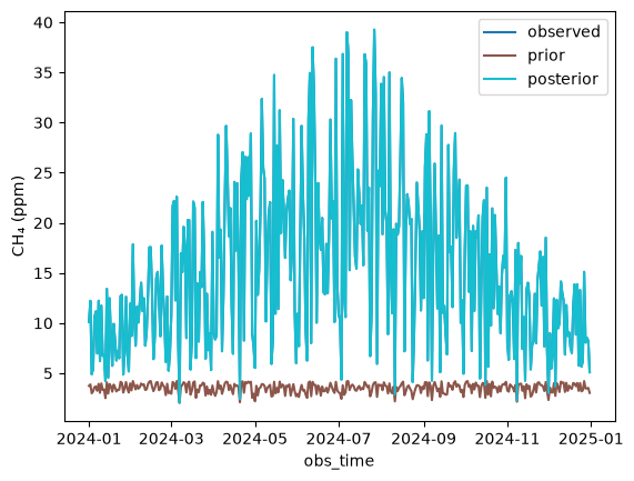
The observations, what the prior predicts and what the estimate predicts, at one site over the year.

def at_site(vector, name, site="site_a"):
    """Return one site's concentrations over time, as a Series named for the legend."""
    return vector.to_series().droplevel("block").xs(site, level="site").rename(name)


fig, ax = plot_comparison(
    at_site(problem.obs, "observed"),
    at_site(problem.predict(problem.prior), "prior"),
    at_site(post.modeled_obs, "posterior"),
)
ax.set_ylabel("CH₄ (ppm)");

Monthly totals and their uncertainty

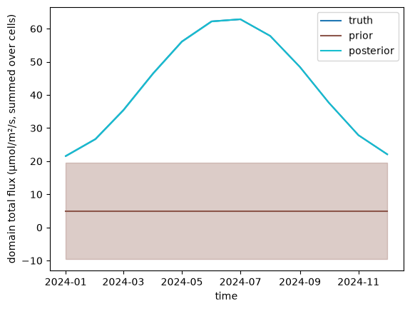
The question is often about an aggregate: the flux summed over the domain each month. fips.aggregate.sum builds the aggregation, and post.cov(W) is the posterior covariance of the totals, computed without the full 1200 x 1200 posterior covariance. plot_comparison draws the prior and the posterior with a band of one standard deviation each, and the truth.

W = fips.aggregate.sum(prior.space, by="time")


def total(vector, name):
    """Return the domain total of each month, as a Series named for the legend."""
    return (W @ vector).to_series().droplevel("block").rename(name)


fig, ax = plot_comparison(
    total(truth, "truth"),
    total(problem.prior, "prior"),
    total(post.estimate, "posterior"),
    errors=[None, W @ problem.prior_cov @ W.T, post.cov(W)],
)
ax.set_ylabel("domain total flux (µmol/m²/s, summed over cells)");

Which months the data constrain

The averaging kernel of the totals says how the estimated total of each month responds to its true total: near 1 where the observations decide it, near 0 where it stays at the prior. Here every month is decided by the data (each has about 90 observations), so the table is the identity matrix; a -0.0 is a tiny negative number, rounded.

post.averaging_kernel(W).to_frame().round(2)

	block	flux
	time	2024-01-01	2024-02-01	2024-03-01	2024-04-01	2024-05-01	2024-06-01	2024-07-01	2024-08-01	2024-09-01	2024-10-01	2024-11-01	2024-12-01
block	time
flux	2024-01-01	1.0	0.0	0.0	-0.0	-0.0	0.0	-0.0	0.0	0.0	-0.0	-0.0	-0.0
	2024-02-01	0.0	1.0	0.0	0.0	-0.0	0.0	-0.0	-0.0	0.0	-0.0	0.0	-0.0
	2024-03-01	0.0	0.0	1.0	0.0	0.0	0.0	-0.0	0.0	0.0	-0.0	0.0	-0.0
	2024-04-01	0.0	0.0	0.0	1.0	0.0	0.0	0.0	0.0	0.0	-0.0	0.0	-0.0
	2024-05-01	0.0	0.0	0.0	0.0	1.0	0.0	0.0	0.0	0.0	-0.0	0.0	-0.0
	2024-06-01	0.0	0.0	0.0	0.0	0.0	1.0	0.0	0.0	0.0	-0.0	0.0	-0.0
	2024-07-01	0.0	0.0	0.0	0.0	-0.0	0.0	1.0	0.0	0.0	-0.0	0.0	-0.0
	2024-08-01	0.0	0.0	0.0	0.0	-0.0	0.0	0.0	1.0	0.0	0.0	0.0	0.0
	2024-09-01	-0.0	0.0	0.0	0.0	-0.0	0.0	0.0	0.0	1.0	0.0	0.0	0.0
	2024-10-01	-0.0	0.0	0.0	-0.0	-0.0	0.0	0.0	0.0	0.0	1.0	0.0	0.0
	2024-11-01	-0.0	0.0	0.0	-0.0	-0.0	0.0	0.0	0.0	0.0	0.0	1.0	0.0
	2024-12-01	-0.0	0.0	0.0	-0.0	-0.0	0.0	0.0	0.0	0.0	0.0	0.0	1.0