Gravity: density below the surface

Gravity measured along a line at the surface depends on how dense the ground is below it. This notebook finds the density anomaly of 40 buried prisms (a 10 x 4 grid, 1000 m across and 25 to 250 m deep) from the vertical gravity measured at 41 points above them.

In the words of the terminology:

• the state is the density anomaly of each prism (g/cm³);

• the observations are the gravity anomalies at the surface (mGal);

• the forward operator is Newton’s law for a rectangular prism: the gravity at each point from a unit density in each prism;

• the prior is no anomaly anywhere, with a prior covariance that makes neighboring prisms alike, and the observation covariance says the measurements are good to 1% of the largest signal.

import matplotlib.pyplot as plt
import numpy as np
import pandas as pd

import fips
from fips.visualization import plot_comparison

The data and the geometry

The observed gravity anomalies, and where the prisms are.

gravity = np.array(
    [
        6.5112333e-03,
        7.1144759e-03,
        7.8050213e-03,
        8.6004187e-03,
        9.5228049e-03,
        1.0600394e-02,
        1.1869543e-02,
        1.3377636e-02,
        1.5187140e-02,
        1.7381291e-02,
        2.0071869e-02,
        2.3409173e-02,
        2.7592423e-02,
        3.2872699e-02,
        3.9524661e-02,
        4.7739666e-02,
        5.7427097e-02,
        6.8126652e-02,
        7.9261565e-02,
        9.0330964e-02,
        1.0070638e-01,
        1.0950167e-01,
        1.1588202e-01,
        1.1936106e-01,
        1.1961197e-01,
        1.1617789e-01,
        1.0868957e-01,
        9.7370419e-02,
        8.3429883e-02,
        6.9002570e-02,
        5.6079733e-02,
        4.5525921e-02,
        3.7267881e-02,
        3.0880404e-02,
        2.5919366e-02,
        2.2024198e-02,
        1.8925481e-02,
        1.6427182e-02,
        1.4387142e-02,
        1.2701558e-02,
        1.1293783e-02,
    ]
)  # mGal
stations = np.linspace(0, 1000, len(gravity))  # where gravity was measured, m

x_edges = np.linspace(0, 1000, 11)  # the prisms' edges across, m
depth_edges = np.linspace(25, 250, 5)  # and down, m
x_centers = (x_edges[:-1] + x_edges[1:]) / 2
depth_centers = (depth_edges[:-1] + depth_edges[1:]) / 2

Labels and vectors

fips keeps a label beside every number. Each prism is labeled by where it is, its x and its depth; each observation by its x. A Vector is values on such labels: the prior is no anomaly in any prism, in a block named density, and the observations are a block named gravity.

prisms = pd.MultiIndex.from_product([x_centers, depth_centers], names=["x", "depth"])
prior = fips.Vector.from_series(
    pd.Series(0.0, index=prisms, name="prior"), block="density"
)

points = pd.Index(stations, name="x")
obs = fips.Vector.from_series(
    pd.Series(gravity, index=points, name="observed"), block="gravity"
)
prior.space

Space(density: 40 x ['x', 'depth'])

The forward operator

The gravity of a rectangular prism of unit density has a closed form. The matrix has one row per observation and one column per prism, in the order of the labels above (x outer, depth inner), so fips.Operator puts the observations’ labels on its rows and the prisms’ on its columns.

G = 6.67e-4  # the gravitational constant, in units that give mGal


def prism_integral(dx, dz):
    """Return the indefinite integral of the vertical gravity of a 2D prism."""
    return dz * np.arctan(dx / dz) + dx / 2 * np.log(dz**2 + dx**2)


def prism_gravity(stations, x_edges, depth_edges):
    """Return the gravity at each station of a unit density in each prism (stations x prisms)."""
    columns = []
    for x1, x2 in zip(x_edges[:-1], x_edges[1:], strict=True):
        for z1, z2 in zip(depth_edges[:-1], depth_edges[1:], strict=True):
            a, b = x1 - stations, x2 - stations
            columns.append(
                2
                * G
                * (
                    prism_integral(b, z2)
                    - prism_integral(b, z1)
                    - prism_integral(a, z2)
                    + prism_integral(a, z1)
                )
            )
    return np.column_stack(columns)


forward = fips.Operator(
    prism_gravity(stations, x_edges, depth_edges), obs.space, prior.space
)
forward.shape

(41, 40)

The covariances

Neighboring prisms should be alike: the prior covariance correlates two prisms by their distance across (over 200 m) and in depth (over 100 m), with a standard deviation of 0.5 g/cm³. It is a Kronecker product of two exponential correlations, kept as its two small factors. The observations’ errors are independent, at 1% of the largest signal.

prior_cov = fips.Kronecker(
    fips.Exponential("x", 200.0), fips.Exponential("depth", 100.0)
).with_std(0.5)
obs_cov = fips.Independent().with_std(0.01 * gravity.max())

The problem and its solution

A Problem puts the inputs together and checks that every label matches. fips.solve returns the Posterior: the estimate, its uncertainty and the diagnostics of the solve.

problem = fips.Problem(
    prior=prior, prior_cov=prior_cov, obs=obs, obs_cov=obs_cov, forward=forward
)
post = fips.solve(problem)
post.summary()

	gamma	n_state	n_obs	dofs	information_content	chi2	reduced_chi2	r2	rmse	uncertainty_reduction
0	1.0	40	41	16.05898	53.145823	2.723385	0.066424	0.999982	0.000162	0.456763

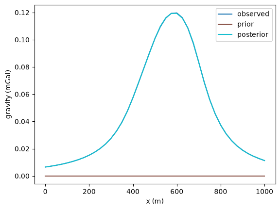
The DOFS say how many independent pieces of information the 41 measurements give about the 40 prisms. The reduced chi-squared is near 1 when the covariances fit the data; here it is well below, because these synthetic observations have no noise at all.

The fit to the data

plot_comparison draws the observations, what the prior predicts (problem.predict, the forward operator times the prior) and what the estimate predicts (post.modeled_obs) on one axes.

def named(vector, name):
    """Return a vector of one block as a Series on its own labels, named for the legend."""
    return vector.to_series().droplevel("block").rename(name)


fig, ax = plot_comparison(
    named(problem.obs, "observed"),
    named(problem.predict(problem.prior), "prior"),
    named(post.modeled_obs, "posterior"),
)
ax.set(xlabel="x (m)", ylabel="gravity (mGal)");

The density below

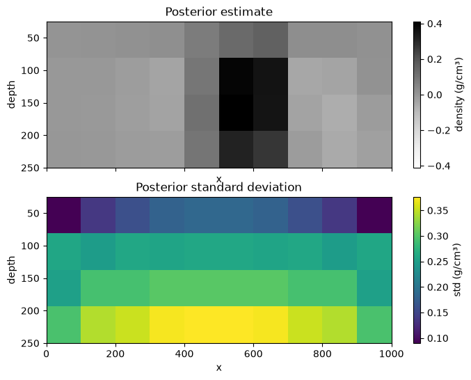
The estimate and its standard deviation, as maps of the prisms: to_xarray() puts a block on its levels, x and depth.

estimate = post.estimate["density"].to_xarray()
std = np.sqrt(post.variances["density"].to_xarray())

fig, axes = plt.subplots(2, 1, figsize=(8, 6), sharex=True)
estimate.plot(
    ax=axes[0],
    x="x",
    y="depth",
    yincrease=False,
    cmap="Greys",
    cbar_kwargs={"label": "density (g/cm³)"},
)
axes[0].set_title("Posterior estimate")
std.plot(
    ax=axes[1],
    x="x",
    y="depth",
    yincrease=False,
    cmap="viridis",
    cbar_kwargs={"label": "std (g/cm³)"},
)
axes[1].set_title("Posterior standard deviation");

How much to trust the data

The regularization factor gamma divides the observation covariance: above 1 the solve trusts the data more, below 1 the prior. The posterior keeps its factorization, so with_gamma gives each gamma’s posterior without solving again, and the rows of summary() stack into a table.

pd.concat(
    [post.with_gamma(g).summary() for g in (0.1, 0.3, 1.0, 3.0, 10.0)],
    ignore_index=True,
)

	gamma	n_state	n_obs	dofs	information_content	chi2	reduced_chi2	r2	rmse	uncertainty_reduction
0	0.1	40	41	12.410882	36.968706	1.221866	0.029802	0.999911	0.000363	0.391886
1	0.3	40	41	13.865537	44.159710	1.808107	0.044100	0.999946	0.000282	0.419185
2	1.0	40	41	16.058980	53.145823	2.723385	0.066424	0.999982	0.000162	0.456763
3	3.0	40	41	18.042533	62.528799	3.426285	0.083568	0.999996	0.000076	0.491897
4	10.0	40	41	19.627809	73.902069	3.867133	0.094320	0.999999	0.000030	0.522448